Hyperparameter optimization with approximate gradient
Chaire Havas-Dauphine
Paris-Dauphine / École Normale Supérieure
Hyperparameters
Most machine learning models depend on at least one hyperparameter to control for model complexity. Examples include:
- Amount of regularization.
- Kernel parameters.
- Architecture of a neural network.
Estimated using some (regularized) goodness of fit on the data.
Cannot be estimated using the same critera as model parameters (overfitting).
Gradient-based hyperparam. optim.
Given a train and a test set, find optimal $\ell_2$ regularization
$$ \begin{aligned} \argmin_{\lambda \in \DD} & ~\testloss(X(\lambda)) \\ \text{s.t. } X(\lambda) = \argmin_{x \in \RR^p} & ~\trainloss(x) + \frac{\lambda}{2} \|x\|^2 \quad. \end{aligned} $$
Hyperparameter optimization as nested or bi-level optimization [J. Domke et al., 2012]
Why not use gradient-based methods to solve this optimization problem?
Gradient-based hyperparam. optim.
How do you compute the gradient of the test loss w.r.t. hyperparameters?
$$ \begin{aligned} \argmin_{\lambda \in \DD} & ~{\text{test_loss}(X(\lambda))} \\ \text{s.t. } X(\lambda) \in \argmin_{x \in \RR^p} & ~\text{train_loss}(x) + \frac{\lambda}{2} \|x\|^2 \quad. \end{aligned} $$
By the chain rule, $$ \nabla_{\lambda} \testloss(\lambda) = \frac{\partial \text{test_loss}}{\partial X} \cdot \underbrace{\frac{\partial X}{\partial \lambda}}_{\text{WTF?}} $$
A way out
Reformulate the inner optimization as an implicit equation (assume e.g. loss is smooth and convex)$ X(\lambda) \in \argmin_{x \in \RR^p} ~\trainloss(x) + \frac{{\lambda}}{2} \|x\|^2 $
$\iff ~\nabla_X \{\underbrace{\testloss(X(\lambda)) + \frac{{\lambda}}{2} \|X(\lambda)\|^2}_{h(\lambda, X(\lambda))}\} = 0 $
- Characterize $X(\lambda)$ as an implicit equation.
- Trick rediscovered many times [J. Larsen 1996, Y. Bengio 2000]
A way out
The original problem can now be written as
$$ \begin{aligned} \argmin_{\lambda \in \DD} & ~{\text{test_loss}(X(\lambda))} \\ \text{s.t. }& \nabla_X h(\lambda, X(\lambda)) = 0 \quad. \end{aligned} $$
Using the formula of implicit differentiation, it is possible to derive a formula for the gradient of the objective function
$$ \nabla_{\lambda} \testloss = - \nabla_X \testloss(X(\lambda)) \cdot \underbrace{(\nabla^2 \trainloss(X(\lambda)) + \lambda I)^{-1} \cdot X(\lambda)}_{\text{costly to compute}} $$
HOAG: hyperparameter optimization with approximate gradient
- Replace $x(\lambda)$ by an approximate solution of the inner optimization.
- Approximately solve linear system.
- Update $\lambda$ using $~~p_k \approx \nabla f$
Tradeoff
Cheap iterations, might diverge.
Costly iterations, convergence to stationary point.
HOAG At iteration $k=1, 2,\ldots$ perform the following:
- i) Solve the inner optimization problem up to tolerance $\varepsilon_k$, i.e. find $x_k \in \RR^p$ such that $$\|{X(\lambda_k) - x_k}\| \leq \varepsilon_k\quad.$$
- ii) Solve the linear system up to tolerance $\varepsilon_k$. That is, find $q_k$ such that$$ \|({\nabla_{1}^2 \trainloss(x_k) + \lambda I) q_k - x_k}\| \leq \varepsilon_k \quad. $$
- iii) Compute approximate gradient $p_k$ as $$ p_k = - \nabla_X \testloss \cdot q_k \quad, $$
- iv) Update hyperparameters: $$ \lambda_{k+1} = P_{\DD}\left(\lambda_k - \frac{1}{L} p_k\right) \quad. $$
Analysis - Global Convergence
Assumptions:
- (A1). $\trainloss$ is $L$-smooth.
- (A2). Hessian of $\trainloss$ is non-singular (or $\lambda > 0$)
- (A3). Domain $\DD$ is bounded (likely superfluous).
Verified e.g. for $\ell_2$-logistic regression, Kernel ridge regression, etc.
Main result: The gradient approximation is bounded for sufficiently large $k$
$$ \| \nabla f(\lambda) - p_k \| = \mathcal{O}(\varepsilon_k) $$
Analysis - Global Convergence
Corollary: If $\{\varepsilon_k\}_{k=1}^\infty$ is a summable,
$\sum_{i=1}^{\infty} \varepsilon_i \lt \infty$,
then $\lambda_k$ converges to a stationary point $\lambda^*$:
$$
\langle \nabla f(\lambda^*), \alpha - \lambda^* \rangle \geq 0 \quad,\quad \forall \alpha \in \DD
$$
$\implies$ if $\lambda^*$ is in the interior of $\DD$ then
$$
\nabla f(\lambda^*) = 0
$$
Corollary: If $\{\varepsilon_k\}_{k=1}^\infty$ is a summable,
$\sum_{i=1}^{\infty} \varepsilon_i \lt \infty$,
then $\lambda_k$ converges to a stationary point $\lambda^*$:
$$
\langle \nabla f(\lambda^*), \alpha - \lambda^* \rangle \geq 0 \quad,\quad \forall \alpha \in \DD
$$
$\implies$ if $\lambda^*$ is in the interior of $\DD$ then $$ \nabla f(\lambda^*) = 0 $$
Implementation - Step size selection.
Adaptive step size (a posteriori)
If $ \testloss(x_k) \leq \testloss(x_{k-1}) + C \varepsilon_k ...$
decrease stepsize: $L = 2 * L$
otherwise
increase it slightly, $L = 0.9 * L$
A posteriori correction of the step size.
Heuristic, don't have an analysis for this step size.
Inspired by adaptive step size strategy in SAG [M. Schmidt et al., 2013]
Experiments
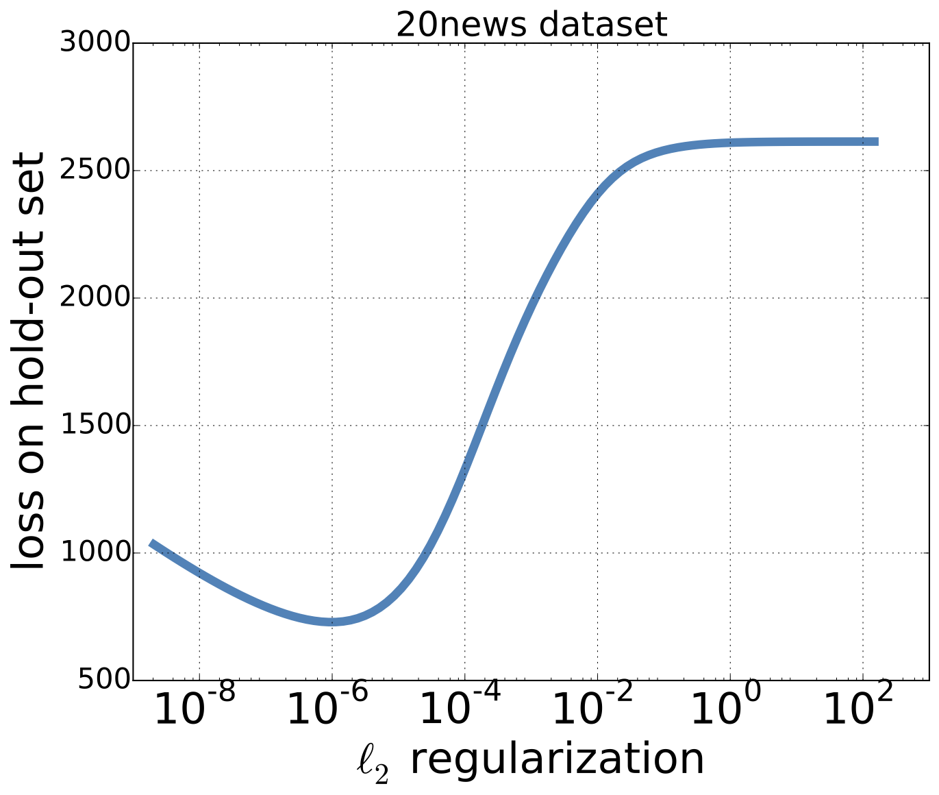
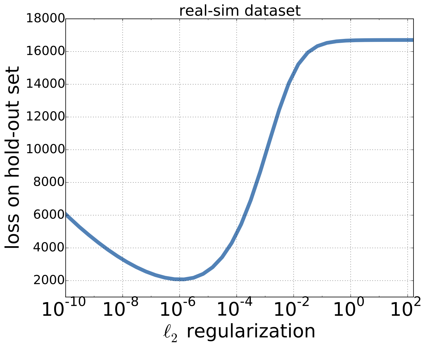
- Model: Logistic regression.
- One hyperparameter: squared $\ell_2$ regularization.
- Cost function $f$: log-likelihood on left-out data.
- Dataset 1: 20news, 11313 samples, 130107 features.
- Dataset 2: real-sim, 62874 samples, 20958 features.
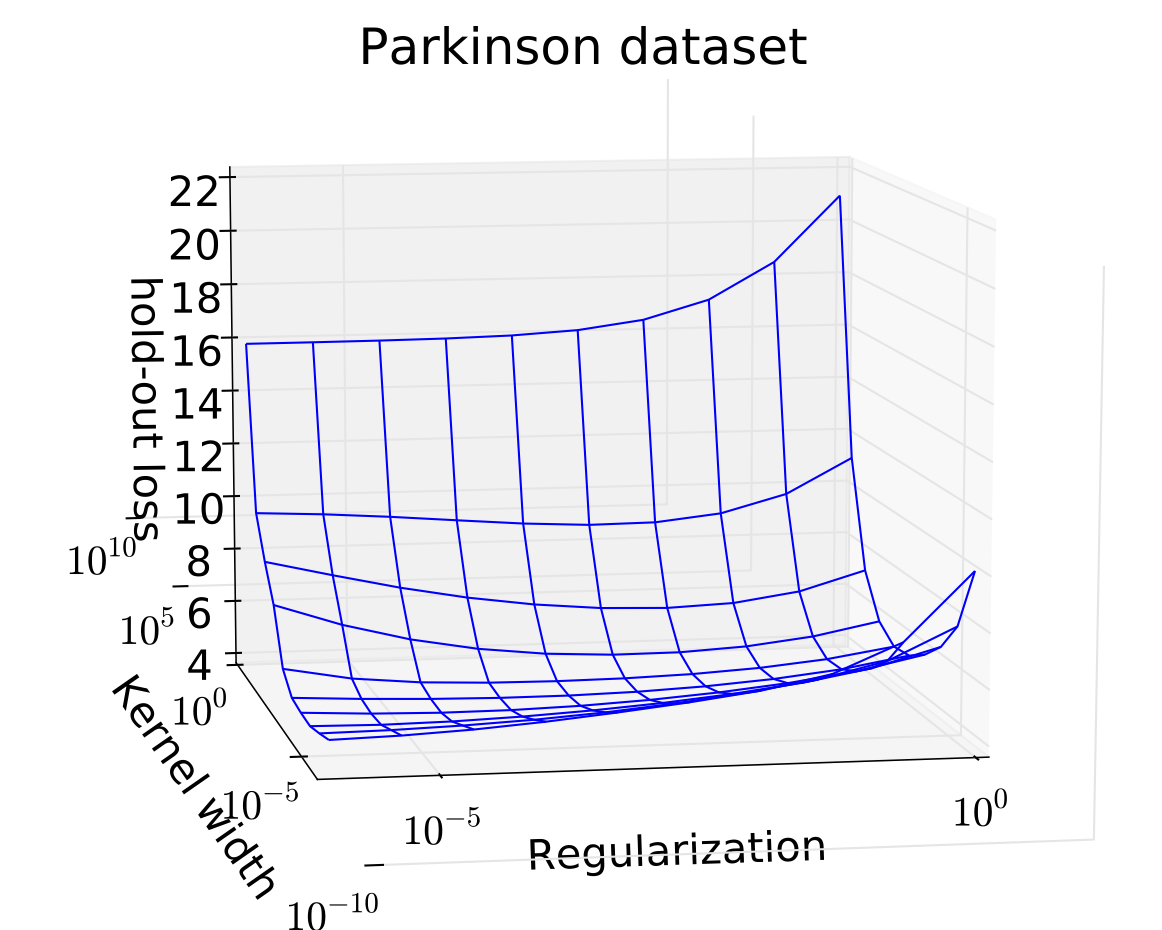
- Model: Kernel ridge regression.
- Two hyperparameter: squared $\ell_2$ regularization.
- Cost function $f$: squared loss on left-out data.
- Dataset: Parkinson 653 samples, 17 features
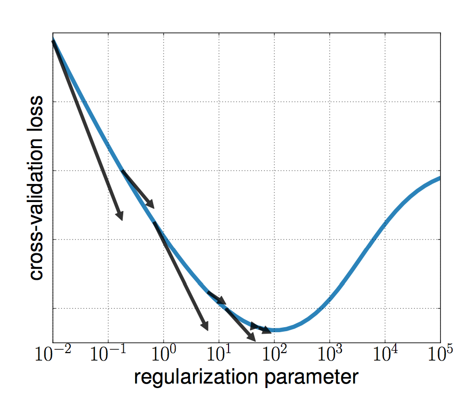
Experiments - cost function
Experiments
How to choose tolerance $\varepsilon^k$?
Different strategies for the tolerance decrease. Quadratic: $\varepsilon(k), \gamma(k) = 0.1 / k^2$, Cubic: $0.1 / k^3$, Exponential: $0.1 \times 0.9^k$
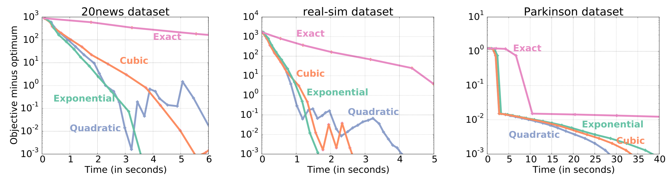
Approximate-gradient strategies achieve much faster decrease in early iterations.