$ \DeclareMathOperator*{\argmin}{arg\,min} \DeclareMathOperator*{\min}{min} \newcommand{\XX}{\mathcal{X}} \newcommand{\RR}{\mathbb{R}} \newcommand{\ff}{\mathbf{f}}$
Feature extraction and supervised learning on fMRI:
from practice to theory
Fabian Pedregosa-Izquierdo, Parietal/Sierra (INRIA)
| Advisors |
Francis Bach |
INRIA/ENS, Paris, France. |
|
Alexandre Gramfort |
Telecom Paristech, Paris, France. |
| Reviewers |
Dimitri Van de Ville |
Univ. Geneva / EPFL, Geneva, CH. |
|
Alain Rakotomamonjy |
University of Rouen, Rouen, France. |
| Examiners |
Ludovic Denoyer |
UPMC, Paris, France. |
|
Marcel A.J. van Gerven |
Donders Institute/Radboud Univ., NL. |
|
Bertrand Thirion |
INRIA/CEA, Saclay, France. |
Dear President of the jury, dear members of the jury, dear audience (friends and colleages). I am pleased to present today an overview of my thesis manuscript entitled "Feature extraction and supervised learning on fMRI: from practice to theory". This work has been accomplished at the Parietal team within the NeuroSpin research center.
Study of cognitive function
Before the advent of non-invasive imaging modalities.
Patients
Lesions

Post-mortem analysis
Finding
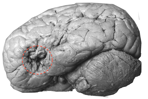
Post-mortem analysis of “Tan” [Paul Broca, 1861]
Until the 20th century most knowledge about the brain came from the study of lesions and post-mortem analysis.
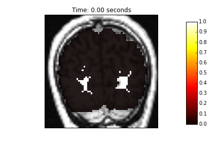
fMRI-based study


Blood-oxygen-level dependent (BOLD) signal
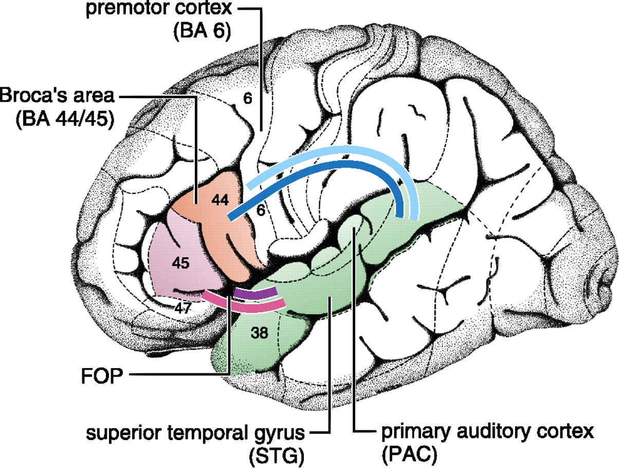
Friederici, A. D. (2011) “The brain basis of language processing: from structure to function”. Physiological reviews
Nowadays, with the advent of non-invasive imaging techniques, notably that of functional MRI, it is possible to study brain function in healthy subjects with a much higher level of precision that was ever possible. The dominant paradigm in this setting is that of task-based fMRI, in which the subjects.
fMRI-based study
Blood-oxygen-level dependent (BOLD) signal
- Processing pipeline
- Preprocessing
- Feature Extraction
- Univariate Statistics
- Supervised Learning
Answer increasingly complex cognitive questions.

E. Cauvet, “Traitement des structures syntaxiques dans le langage et dans la musique”, PhD thesis.
Today, one of the most used method to understand the neural substrate of cognitive functions is task-based fMRI. In this setting, in order to comfront a cognitive hypothesis, a subject is introduced in the scanner while presented some stimuli. During this time, a set of brain images are acquired. The signal acquired in these images is known as the Blood-oxygen-dependent (BOLD) signal, and represents the oxygen consumption at each unit of volume (voxel). These images follow a processing pipeline consisting of several steps before conclusions are drawn. The pipeline consists of several complex steps but also represents exciting oportunities to develop new and better data analysis methods.
Supervised Learning - Decoding
Predict stimuli from activation coefficients.

Contribution: decoding with ordinal values.
We will also focus on the application to supervised learning to fMRI datasets, in a setting known as decoding or reverse inference. In this context, the beta-maps computed in the feature extraction step are used to predict some information about the stimuli. The goal is to establish whether the given prediction is accurate enough to claim that the area encodes some information about the stimuli.
Outline
- 1. Data-driven HRF estimation with R1-GLM.
- Pedregosa, Eickenberg et al. “Data-driven HRF estimation for encoding and decoding models.”, Neuroimage, Jan. 2015.
- Pedregosa, Eickenberg et al. “HRF estimation improves sensitivity of fMRI encoding and decoding models” PRNI 2013
- 2. Decoding with ordinal labels
- Pedregosa et al., “Learning to rank from medical imaging data,” MLMI 2012.
- Pedregosa et al., “Improved Brain Pattern Recovery through Ranking Approaches”, 2012.
- 3. Fisher consistency of ordinal regression models.
- Pedregosa et al., “On the Consistency of Ordinal Regression Methods.”, ArXiv 2014
This talk is divided into 4 parts, corresponding roughly to different chapters of my manuscript
The first part presents a contribution to the step of feature extraction. I will detail a model, named R1-GLM for the joint estimation of HRF and activation coefficients.
In the second part I will move the the supervised learning step of the pipeline and present different methods that can be used to estimate a decoding model when target has a natural ordering.
The General Linear Model (GLM)


where $X_i = \quad \quad~ \ast~ \text{s}_i(t)$
The LTI assumption allows to build a model in which the BOLD is expressed as a linear combination of different regressors multiplied bu the activation coefficients.
Each column of the design matrix contains the HRF convoluted with the stimulus
Basis-constrained HRF
Hemodynamic response function (HRF) is known to vary substantially across subjects, brain regions and age.
D. Handwerker et al., “Variation of BOLD hemodynamic responses across subjects and brain regions and their effects on statistical analyses.,” Neuroimage 2004.
S. Badillo et al., “Group-level impacts of within- and between-subject hemodynamic variability in fMRI,” Neuroimage 2013.
Two basis-constrained models of the HRF: FIR and 3HRF.
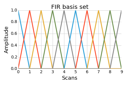
In the GLM just introduced, the HRF is assumed to be known. However, it is known that the HRF varies substantially across
In this setting the HRF is assumed to be a linear combination elements in a set of basis functions.
R1-GLM

(
$\beta_1$$h_1$
$\beta_1$$h_2$
$\beta_1$$h_3$
$\beta_2$$h_4$
$\beta_2$$h_5$
$\beta_2$$h_6$ $\cdots$
$\beta_{k}$$h_{3k-2}$
$\beta_{k}$$h_{3k-1}$
$\beta_k$$h_{3k}$)
$ = \mathbf{h} \boldsymbol{\beta}^T$
Estimated as the solution to the optimization problem
$ \argmin_{\mathbf{h}, ~\boldsymbol{\beta}} \|\mathbf{y} - \mathbf{X} \text{vec}(\mathbf{h}\boldsymbol{\beta}^T)\|^2$
subject to $\|\ \mathbf{h}\| = 1$ and $\langle \mathbf{h}, \mathbf{h}_{\text{ref}} \rangle > 0$.
$\implies$ solved locally using quasi-Newton methods.
The resulting model is smooth (albeit non-convex) and can be solved using a variety of methods. The easiest to implement is to alternate the optimization of h and beta, where at each step we have a least squares subproblem. We found however that a joint minimization on both vectors is much faster using gradient-based methods.
Validation of R1-GLM

- Improvement using decoding and encoding models.
Ground truth unknown. HRF often a nuisance parameter in neuroimaging studies. Since we don't have access to the ground truth we look for alternate measures that can assess. Why you validate like this ?
Results
Cross-validation score in two different datasets
S. Tom et al., “The neural basis of loss aversion in decision-making under risk,” Science 2007.
K. N. Kay et al., “Identifying natural images from human brain activity.,” Nature 2008.
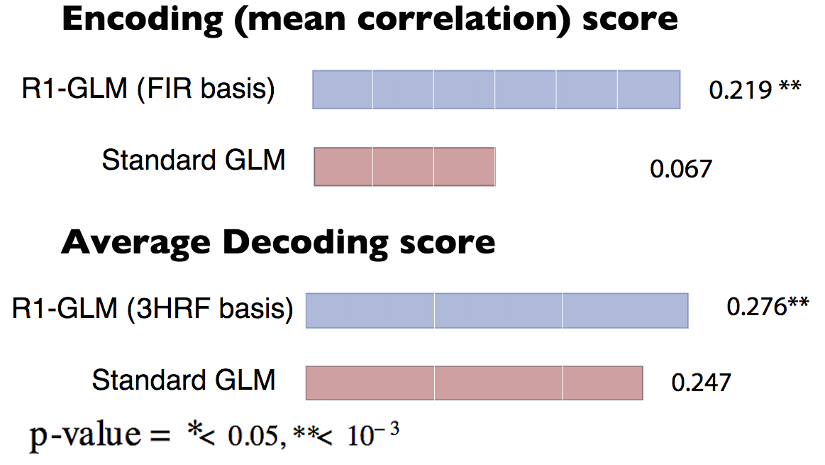
Results - Encoding
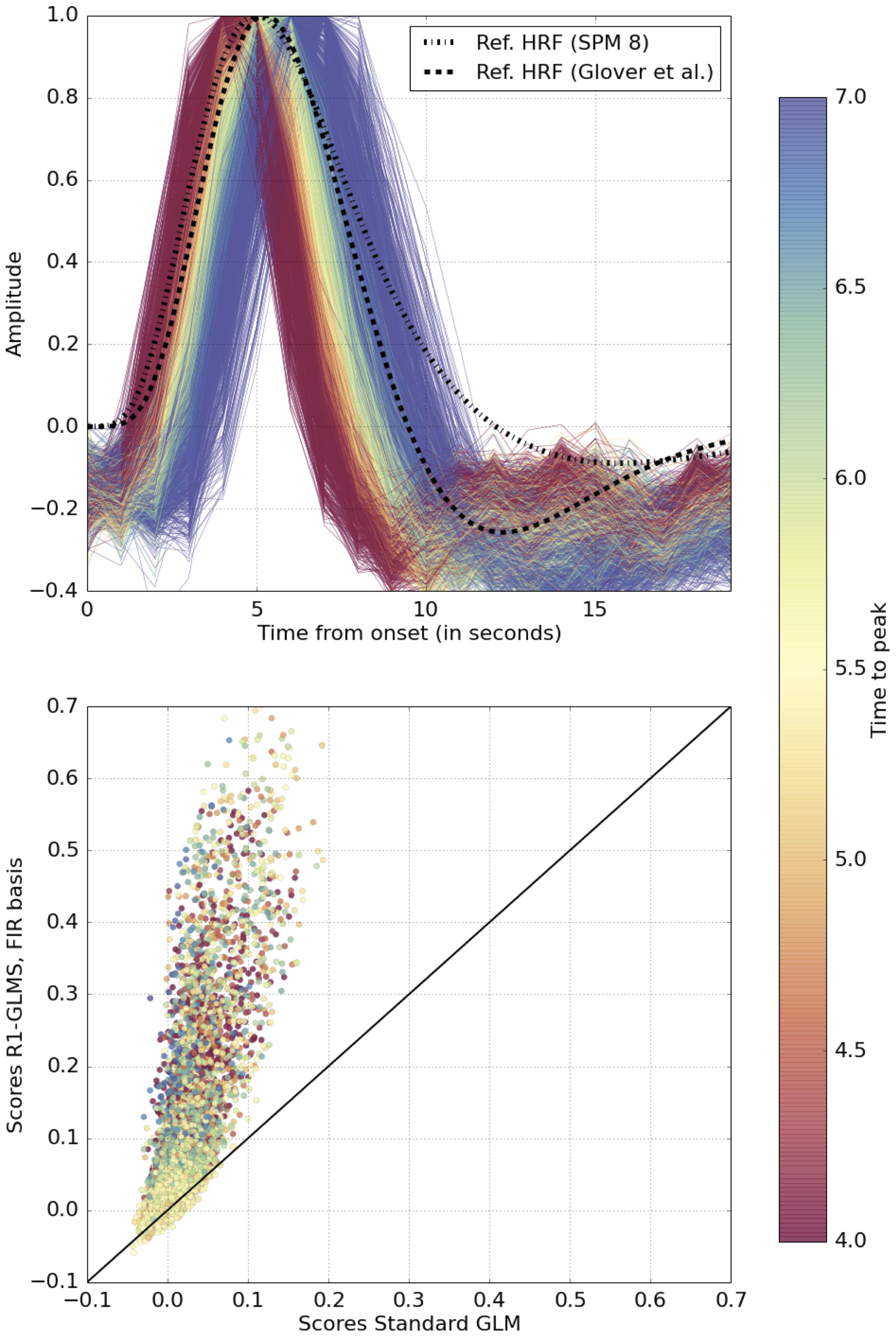
- Measure: voxel-wise encoding score. Correlation with the BOLD at each voxel on left-out data.
- R1-GLM (FIR basis) improves voxel-wise encoding score on more than 98% of the voxels.
Conclusions
- Model for the joint estimation of HRF and activation coefficients.
- Constrained estimation of the HRF while remaining computationally tractable (~1h for full brain estimation).
- Validated the pertinence of this model by improvement in decoding and encoding score obtained on two fMRI datasets.
- Article and software distribution
- “Data-driven HRF estimation for encoding and decoding models.,” Pedregosa, Eickenberg et al., Neuroimage, Jan. 2015.
- hrf_estimation: http://pypi.python.org/pypi/hrf_estimation
Outline
- 1. Data-driven HRF estimation with R1-GLM.
- Pedregosa, Eickenberg et al. “Data-driven HRF estimation for encoding and decoding models.”, Neuroimage, Jan. 2015.
- Pedregosa, Eickenberg et al. “HRF estimation improves sensitivity of fMRI encoding and decoding models” PRNI 2013
- 2. Decoding with ordinal labels
- Pedregosa et al., “Learning to rank from medical imaging data,” MLMI 2012.
- Pedregosa et al., “Improved Brain Pattern Recovery through Ranking Approaches”, 2012.
- 3. Fisher consistency of ordinal regression models.
- Pedregosa et al., “On the Consistency of Ordinal Regression Methods.”, ArXiv 2014
This talk is divided into 4 parts, corresponding roughly to different chapters of my manuscript
The first part presents a contribution to the step of feature extraction. I will detail a model, named R1-GLM for the joint estimation of HRF and activation coefficients.
In the second part I will move the the supervised learning step of the pipeline and present different methods that can be used to estimate a decoding model when target has a natural ordering.
Decoding with ordinal labels
$\mathbf{X} \quad \to \quad \mathbf{y}$
Activation coefficients
Target values
Target values can be
- Binary $\{-1, 1\}$
- Continuous $\{0.34, 1,3, \ldots \}$
- Ordinal: $\{1, 2, 3, \ldots, k\}$, $1 \prec 2 \prec 3$ ...
How can we incorporate the order information into a decoding model ?
We now enter the second part of this presentation entitled decoding with ordinal labels. This is motivated by the need to analyze different fMRI datasets in which the target variable consist of ordinal values, as it arised within the work of different colleages at NeuroSpin.
The first dataset that we would like to analyze is a dataset in which the target variable consists of phrases with different levels of complexity.
Loss functions
Two relevant loss functions:
- $\ell_{\mathcal{A}}(y, \hat{y}) = | y - \hat{y}|$.
- Measures the distance betwen the predicted and true label.
- Models: Ordinal Logistic Regression, Least Absolute Error, Cost-sensitive Multiclass
- $ \ell_{\mathcal{P}}(y_1, y_2, \hat{y}_1, \hat{y}_1) =$ 0 if $\text{sign}(y_1-y_2)$ = $\text{sign}(\hat{y}_1 - \hat{y}_2))$, 1 otherwise.
- Measures ordering betweem $(y_1, y_2)$ and $(\hat{y}_1, \hat{y}_2)$.
- Models: LogisticRank
2 loss functions $\implies$ 2 aspects of the ordinal problem.
Since we are going to compare models, we first need to choose an evaluation metric, that is, the function that we will use to compare the different models.
Ordinal Logistic Regression
- J. Rennie and N. Srebro, “Loss Functions for Preference Levels : Regression with Discrete Ordered Labels,” IJCAI 2005.

Generalization of logistic regression.
Parameters ($p$ = num. dimensions, $k$ = num. classes)
- coefficients $\mathbf{w} \in \RR^p$
- non-decreasing thresholds: $\boldsymbol{\theta} \in \RR^{k-1}$
Prediction
1 + $\argmin\{i: \mathbf{w}^T \mathbf{x} > \theta_i \}$
Surrogate loss function:
$\sum_{j=1}^{y-1} \text{logistic}(\theta_j-\mathbf{w}^T \mathbf{x}) + \sum_{j=y}^{k-1} \text{logistic}(\mathbf{w}^T \mathbf{x} - \theta_j)$
Pairwise ranking
- R. Herbrich et al., “Support Vector Learning for Ordinal Regression,” 1999.
- T. Joachims, “Optimizing Search Engines using Clickthrough Data,” SIGKDD 2002.
Parameters ($p$ = num. dimensions, $k$ = num. classes)
- coefficients $\mathbf{w} \in \RR^p$
Prediction: $\text{sign} (\mathbf{w}^T \mathbf{x}_i - \mathbf{w}^T\mathbf{x}_j) = \text{sign} (\mathbf{w}^T(\mathbf{x}_i - \mathbf{x}_j))$
Surrogate loss function
$\text{logistic} (\text{sign}(y_i - y_j)(\mathbf{w}^T (\mathbf{x}_i - \mathbf{x}_j)))$
$\implies$ can be implemented as a binary-class logistic regression model, $\hat{y}_{ij} = y_i - y_j, \hat{\mathbf{x}}_{ij} = \mathbf{x}_i - \mathbf{x}_j$
This loss was first proposed within the context of information retrieval.
Two fMRI datasets, three tasks
1) Predict level of complexity of a phrase (6 levels)
E. Cauvet, Traitement des structures syntaxiques dans le langage et dans la musique, PhD thesis
2) Predict number of letters in a word.
3) Predict real size of objects from noun.
V. Borghesani, “A perceptual-to-conceptual gradient of word coding along the ventral path,” PRNI 2014.

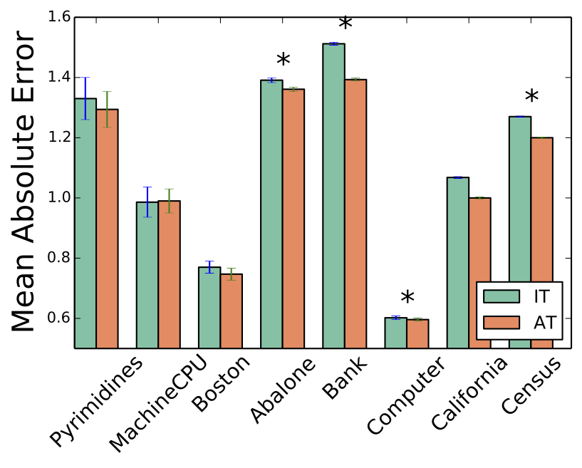
Results - Mean Absolute Error
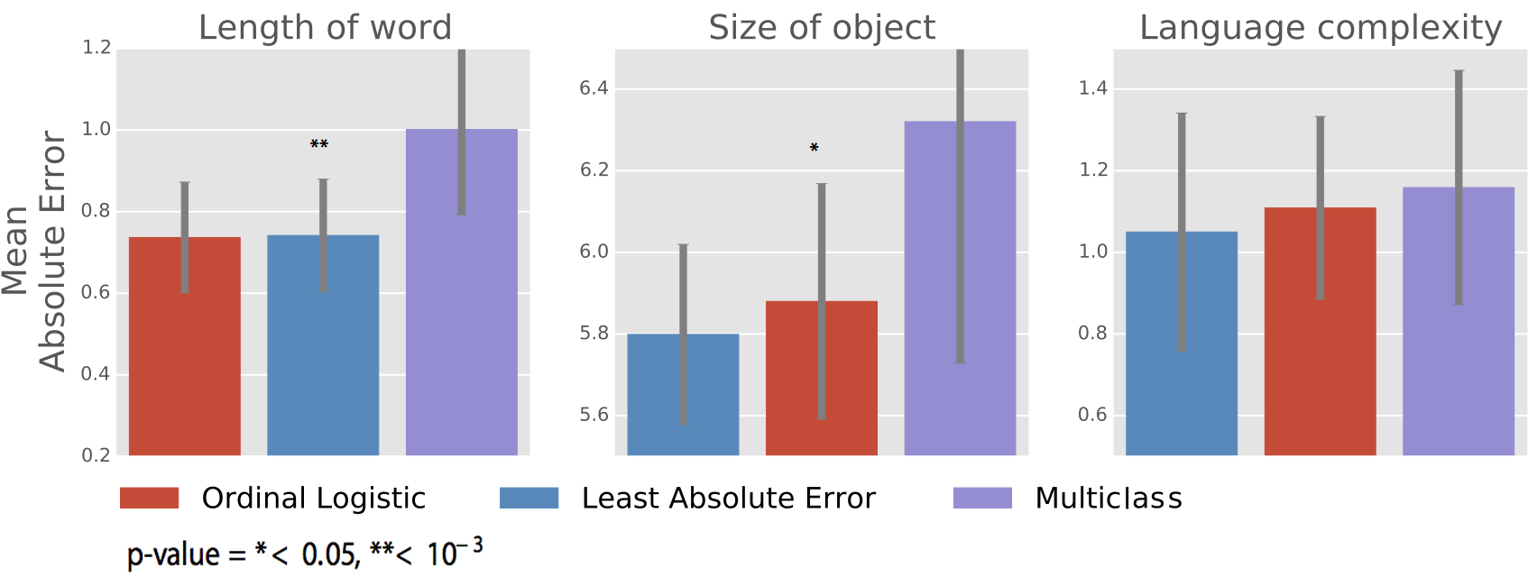
Top performers:
- Ordinal Logistic
- Least Absolute Error.
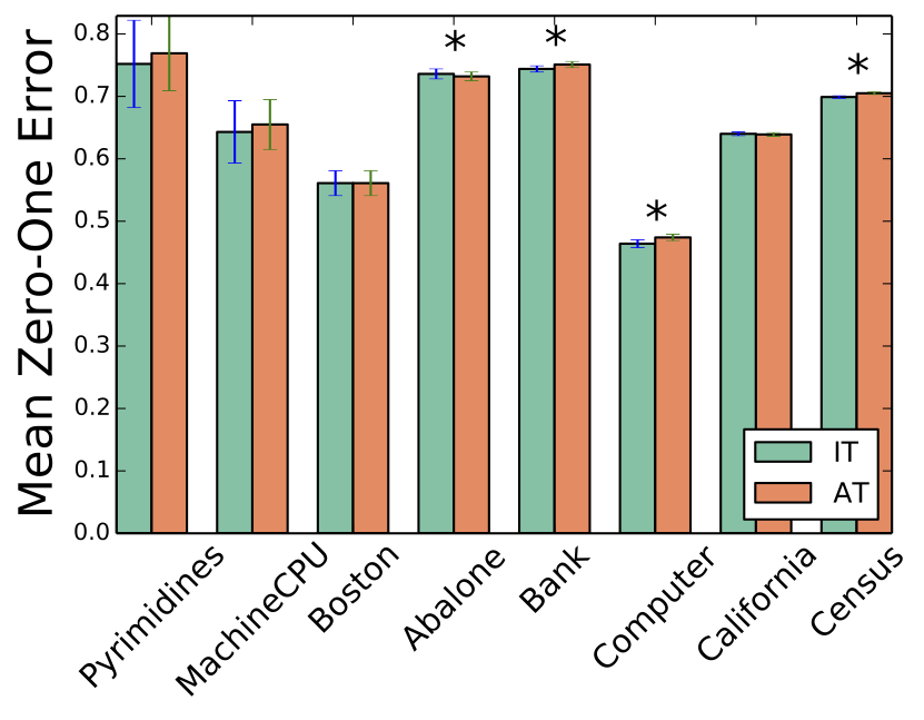
Results - Pairwise Disagreement
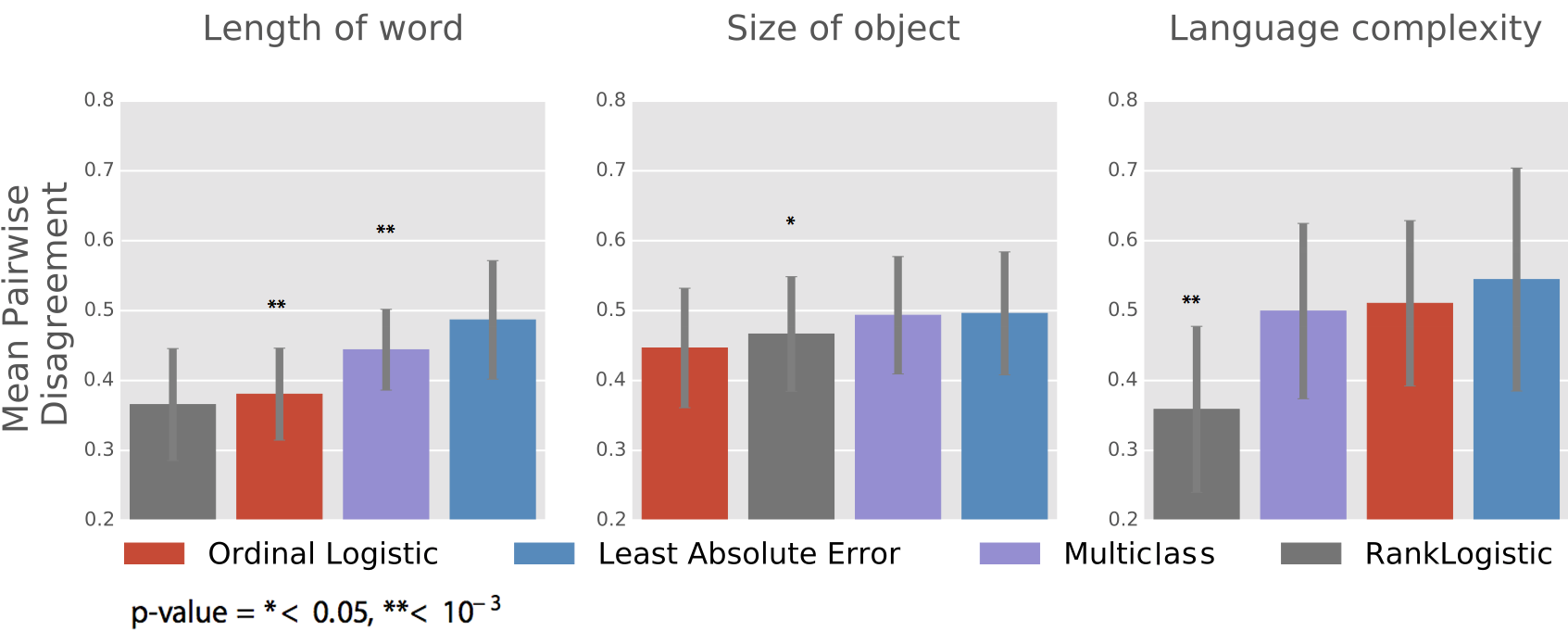
Top performer: RankLogistic
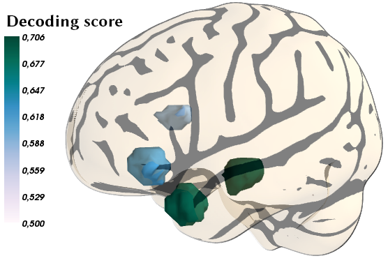
Application: role of language ROIs in complexity of sentences.
F. Pedregosa et al., “Learning to rank from medical imaging data,” MLMI 2012.
Conclusions
- Two loss functions for the task of decoding with ordinal values.
- Using 4 different models, use order information in context of fMRI-based brain decoding.
- Benchmarked the methods on 3 tasks (2 datasets).
- First usage of pairwise ranking in the context of fMRI, software distribution.
- “Learning to rank from medical imaging data,” Pedregosa et al. MLMI 2012.
- PySofia: https://pypi.python.org/pypi/pysofia
Outline
- 1. Data-driven HRF estimation with R1-GLM.
- Pedregosa, Eickenberg et al. “Data-driven HRF estimation for encoding and decoding models.”, Neuroimage, Jan. 2015.
- Pedregosa, Eickenberg et al. “HRF estimation improves sensitivity of fMRI encoding and decoding models” PRNI 2013
- 2. Decoding with ordinal labels
- Pedregosa et al., “Learning to rank from medical imaging data,” MLMI 2012.
- Pedregosa et al., “Improved Brain Pattern Recovery through Ranking Approaches”, 2012.
- 3. Fisher consistency of ordinal regression models.
- Pedregosa et al., “On the Consistency of Ordinal Regression Methods.”, ArXiv 2014
This talk is divided into 4 parts, corresponding roughly to different chapters of my manuscript
The first part presents a contribution to the step of feature extraction. I will detail a model, named R1-GLM for the joint estimation of HRF and activation coefficients.
In the second part I will move the the supervised learning step of the pipeline and present different methods that can be used to estimate a decoding model when target has a natural ordering.
Ordinal Regression surrogates
- IT) ${\text{logistic}}(f(X) - \theta_{y-1}) + {\text{logistic}}(\theta_{y} - f(X))$
- AT) $\sum_{i=1}^{y-1}{\text{logistic}}(f(X) - \theta_{i}) + \sum_{i=y}^k {\text{logistic}}(\theta_{i} - f(X))$
- J. Rennie and N. Srebro, “Loss Functions for Preference Levels : Regression with Discrete Ordered Labels,” IJCAI 2005.
- IT) ${\color{BlueViolet}\text{hinge}}(f(X) - \theta_{y-1}) + {\color{BlueViolet}\text{hinge}}(\theta_{y} - f(X))$
- AT) $\sum_{i=1}^{y-1} {\color{BlueViolet}\text{hinge}}(f(X) - \theta_{i}) + \sum_{i=y}^k {\color{BlueViolet}\text{hinge}}(\theta_{i} - f(X))$
- W. Chu and S. S. Keerthi, “New approaches to Support Vector Ordinal Regression,” ICML 2005.
- IT) ${\color{BlueViolet}\text{exp}}(-(f(X) - \theta_{y-1})) + {\color{BlueViolet}\text{exp}}(-(\theta_{y} - f(X)))$
- AT) $\sum_{i=1}^{y-1}{\color{BlueViolet}\text{exp}}(-(f(X) - \theta_{i})) + \sum_{i=y}^k {\color{BlueViolet}\text{exp}}(-(\theta_{i} - f(X)))$
- H. Lin and L. Li, “Large-Margin Thresholded Ensembles for Ordinal Regression : Theory and Practice,” Algorithmic Learning Theory 2006.
Empirical comparison
- [Rennie & Srebro 2005]
- [Chu & Keerthi 2005]
- [Lin & Li 2006]
Is there a reason that can explain this behaviour ?
Mean Absolute Error
So according to these studies it seems that that loss functions of the form b) perform better on the datasets they tried. Question: should we assume that because it performed better on some datasets b) is superior to a) ?.
The results that we will give in this section provide theoretical insight on this question.
Fisher consistency
- Goal supervised learning: minimize risk : \begin{equation} \label{eq:l_risk} \mathcal{R}_{\ell}(h) = \mathbb{E}(\ell(Y, h(X)))\quad. \end{equation}
- $\implies$ computationally intractable. Minimize the surrogate risk$$\mathcal{R}_{\psi}(h) = \mathbb{E}(\psi(Y, h(X)))$$
Fisher consistency:
- Relate minimizer of $\mathcal{R}_{\psi}$ with the minimizer of $\mathcal{R}_{\ell}$.
- $$f^* \in \argmin_{f \in \mathcal{F}} \mathcal{R}_{\psi}(f) \implies \mathcal{R}_{\ell}(f^*) = \mathcal{R}_{\ell}(h^*)$$ where $h^*$ is a minimizer of the risk (Bayes rule)
We will now define the supervised learning problem from a probabilistic setting. We will need this to give the definition of Fisher consistency (for surrogate loss functions).
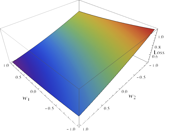
Illustration
Binary-class linear problem on $\RR^2$
- a) $\sum_{i}^n \ell(y_i, h(X_i))$
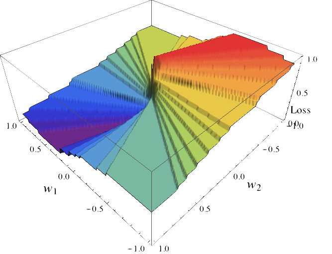
- b) $\sum_{i}^n \text{logistic}(y_i X w))$
Fisher consistency
Previous work
- Binary classification
- P. Bartlett et al., “Convexity , Classification , and Risk Bounds,” J. Am. Stat. Assoc. 2003.
- Pairwise ranking
- J. Duchi et al., “On the Consistency of Ranking Algorithms,” ICML 2010.
- Ordinal Regression
- Pedregosa et al., “On the Consistency of Ordinal Regression Methods.”, ArXiv preprint, Nov. 2014
Fisher consistency is a condition on XXX.
Threshold-based surrogates
Propose a formulation that parametrizes the ordinal regression surrogates seen so far
$$\psi^{\ell}(y, \boldsymbol{\alpha}) = \sum_{i = 1}^{y-1} \Delta \ell(y, i)\phi(\alpha_i) - \sum_{i=y}^{k-1}\Delta \ell(y, i)\phi(-\alpha_i)$$
where
- $\Delta\ell(y, i) = \ell(y,i+1) - \ell(y, i)$
- $\phi: \RR \to \RR$ is a binary-class surrogate loss function (hinge, logistic, etc.).
- For $\ell$ = zero-one loss $\implies$ $\psi^{\ell}$ = Immediate Threshold (IT).
- For $\ell$ = absolute error loss $\implies$ $\psi^{\ell}$ = All Threshold (AT).
Consistency of $\psi^{\ell}$
$\psi^{\ell}(y, \boldsymbol{\alpha}) = \sum_{i = 1}^{y-1} \Delta \ell(y, i)\phi(\alpha_i) - \sum_{i=y}^{k-1}\Delta \ell(y, i)\phi(-\alpha_i)$
- Main result
- ${\phi: \RR \rightarrow \RR_+}$ consistent with respect to the zero-one binary loss, i.e., $\phi$ is differentiable at zero and $\phi'(0) < 0$
- $\implies$ the surrogate $\psi^{\ell}$ is consistent with respect to $\ell$
- IT) ${\phi}(f(X) - \theta_{y-1}) + {\phi}(\theta_{y} - f(X))$ $\implies$ consistent w.r.t. 0-1 loss
- AT) $\sum_{i=1}^{y-1}{\phi}(f(X) - \theta_{i}) + \sum_{i=y}^k {\phi}(\theta_{i} - f(X))$ $\implies$ consistent w.r.t. absolute error
Illustration
- AT performs better w.r.t Absolute Error
- IT performs better w.r.t. Zero-One Error
Other results
Consistency
- Absolute Error surrogate: ($\psi_{\mathcal{A}}(y, \alpha) = |y - \alpha|$)
- Consistent w.r.t. Absolute Error
- Extends results of [H. Ramaswamy 2012]
- Squared Error surrogate: $\psi_{\mathcal{S}}(y, \alpha) = (y - \alpha)^2$
- Consistent w.r.t. Squared Error
- Proportional odds [McCullagh 1980]: $P(y \leq i | X) = \sigma(\theta_i - X w)$
- Consistent w.r.t. Absolute Error
Perspectives
computational cost of R1-GLM
$$\argmin_{\mathbf{h}, ~\boldsymbol{\beta}} \|\mathbf{y} - \mathbf{X} \text{vec}(\mathbf{h}\boldsymbol{\beta}^T)\|^2$$
While the R1-GLM performs much better than the alternative methods, it is my opinion that there is still margin for improvement.
For example, the current optimization algorithm solves many optimization problems of the form XXX and it does not use the information that the X is always the same.
Also, the model is frustratingly similar (but not equivalent!) to that of reduced rank regression [Andersen et al. XXX]
Perspectives
Consistency in a constrained space.
- Current proof implicitly assumes decision functions can be separately defined for each sample.
- Threshold-based decision functions are of the form $(\theta_1 - f(X), \theta_2 - f(X), \ldots, \theta_{k-1} - f(X))$.
- $\boldsymbol{\theta}$ is shared among all samples.
- Is it possible to obtain consistency results in this setting ?
While the R1-GLM performs much better than the alternative methods, it is my opinion that there is still margin for improvement.
For example, the current optimization algorithm solves many optimization problems of the form XXX and it does not use the information that the X is always the same.
Also, the model is frustratingly similar (but not equivalent!) to that of reduced rank regression [Andersen et al.]
Thanks for your attention
Backup slides
The Linear-Time-Invariant assumption
The model of the BOLD signal that is commonly used assumes a linear-time-invariant relationship between the BOLD signal and the neural response.

Source: [Poldrack et al. 2011]
- Homogeneity: If a neural response is scaled by a factor of $a$, then the BOLD response is also scaled by this same factor of $a$.
- Additivity: The response for two separate events is the sum of the independent signals.
- Time invariant: If a stimulus is shifted $t$ seconds, the BOLD response will be shifted by this same amount.
As outlined in the introduction, the estimation of activation coefficients from BOLD signal is challenging due to the delayed nature of the hemodynamic response.
To make the identification problem well posed, it is common to rely on an assumption that relates the BOLD signal to neural activity and that has been empirically shown to hold under a wide range of circumtances. This is known as the linear-time-invariant assumption and is based on the following three points.
HRF variability
- Across age
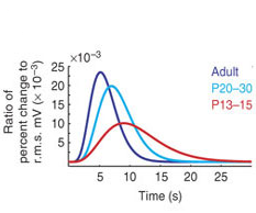
- Across age: Matthew T. Colonnese, et al�. “Development
of hemodynamic responses and functional connectivity in rat somatosensory cortex”. Nature neuroscience 2007
Extension to separate designs
- GLMS: Extension of the classical GLM proposed by [Mumford et al. 2012] that improves estimation in highly correlated designs.
R1-GLM with separate designs: R1-GLMS
Optimization problem of the form
$ \sum_i^k \|\mathbf{y} - \beta_i \mathbf{X}^0_{\text{BS}i} \mathbf{h} - r_i \mathbf{X}^1_{\text{BS}i} \mathbf{h}\| ^2$
Subject to $\|\mathbf{B} \mathbf{h}\|_{\infty} = 1$ and $\langle \mathbf{h}, \mathbf{h}_{\text{ref}} \rangle > 0$
Source: [Mumford et al. 2012]
Recently a variation on the classical GLM was proposed by Mumford et al. that has been shown to improve estimation in highly correlated designs. The technique is simple, for each of the different stimuli, the design matrix is collapsed into two
Results - Encoding


Results - Decoding

Absolute Error
Models: Least Absolute Error, Ordinal Logistic Regression , Multiclass Classification
Least Absolute Error
Model parameters: $\mathbf{w} \in \RR^p, b \in \RR$
Decision function: $f(\mathbf{x}_i) = b + \langle \mathbf{x}_i, \mathbf{w} \rangle$
Prediction: $\text{round}_{1 \leq i \leq k} (f(\mathbf{x}_i))$
Estimation: $\mathbf{w}^*, b^* \in \argmin_{\mathbf{w}, b} \frac{1}{n}\sum_{i=1}^n |y_i - f(\mathbf{x}_i)| + \lambda \|\mathbf{w}\|^2$
Regression model in which the prediction is given by rounding to the closest label.