Quasi-Newton and BFGS
The central issue with Newton's method is that we need to be able to compute the inverse Hessian matrix. For machine learning applications, the dimensionality of the problem can be of the order of thousands or millions. Computing the Hessian or its inverse is often impractical.
Because of these reasons, Newton's method is rarely used in practice to optimize functions corresponding to large problems. Luckily, the above algorithm can still work even if the Hessian is replaced by a good approximation.
In quasi-Newton methods, the Hessian matrix of second derivatives doesn't need to be evaluated directly. Instead, the Hessian matrix is approximated using updates specified by gradient evaluations (or approximate gradient evaluations).
The BFGS algorithm
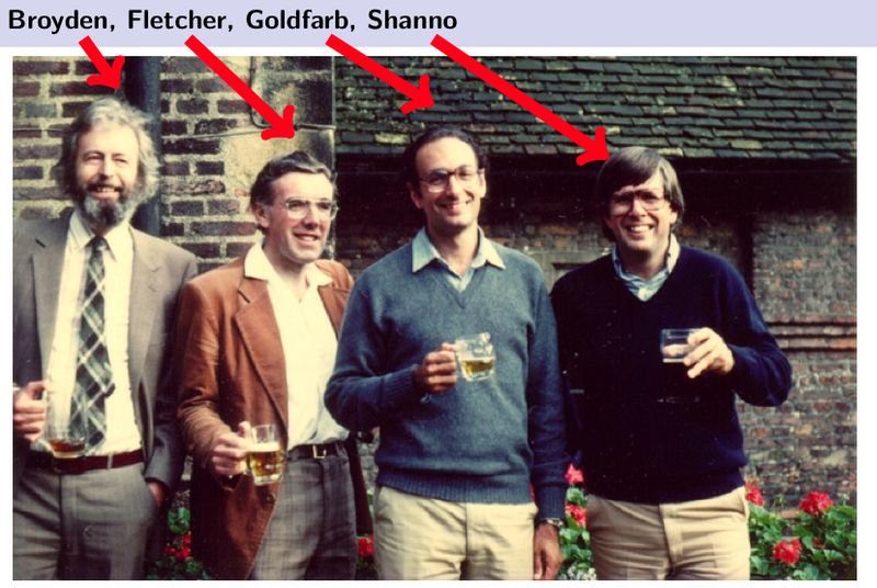
One of the most popular quasi-Newton methods is the BFGS algorithm. The algorithm is named after Charles George Broyden, Roger Fletcher, Donald Goldfarb and David Shanno.

As in the case of Newton's method, we aim to solve the following unconstrained optimization problem
\begin{equation}\label{eq:fw_objective} \minimize_{\boldsymbol{x} \in \RR^p} f(\boldsymbol{x}) ~, \end{equation}
when $f$ is twice differentiable.
Behave like a Hessian
Key idea. As a byproduct of the optimization, we observe many gradients. Can we use these gradients to iteratively construct an estimate of the Hessian?
In this method we consider at each iteration the following surrogate function \begin{equation} Q_t(\xx) = c_t + \boldsymbol{g}_t^T(\xx - \xx_t) + \frac{1}{2 \gamma}(\xx - \xx_t)^T \boldsymbol{H}_t (\xx - \xx_t)~. \end{equation} where in this case $\HH_t$ is an approximation to the Hessian matrix, which is updated iteratively at each stage, and $\nabla f(\xx_t)$ is the gradient of the function evaluated at $\xx_t$.
A reasonable thing to ask to this surrogate is that its gradient coincides with $f$ at the two last iterates $\xx_{t+1}$ and $\xx_{t}$: \begin{align} \nabla Q_{t+1}(\xx_{t+1}) &= \nabla f(\xx_{t+1})\\ \nabla Q_{t+1}(\xx_{t}) &= \nabla f(\xx_{t})\\ & \implies \HH_{t+1} (\xx_{t+1}-\xx_t ) = \nabla f(\xx_{t+1}) - \nabla f(\xx_t ). \end{align}
Let $\mathbf{y}_t = \nabla f(\xx_{t+1}) - \nabla f(\xx_t)$ and $\mathbf{s}_t = \xx_{t+1}-\xx_t$, then $\HH_{t+1}$ satisfies $\HH_{t+1} \mathbf{s}_t = \mathbf{y}_t $ which is the secant equation. The curvature condition $\mathbf{s}_t^\top \mathbf{y}_t > 0$ should be satisfied. If the function is not strongly convex, then the condition has to be enforced explicitly. In order to maintain the symmetry and positive definitiveness of $\HH_{t+1}$, the update form can be chosen as: $\HH_{t+1} = \HH_t + \alpha\mathbf{u}\mathbf{u}^\top + \beta\mathbf{v}\mathbf{v}^\top$. Imposing the secant condition, $\HH_{t+1} \mathbf{s}_t = \mathbf{y}_t $. With this, we get the update equation of $\HH_{t+1}$: \begin{equation} \HH_{t+1} = \HH_t + \frac{\mathbf{y}_t \mathbf{y}_t^{\mathrm{T}}}{\mathbf{y}_t^{\mathrm{T}} \mathbf{s}_t} - \frac{\HH_t \mathbf{s}_t \mathbf{s}_t^{\mathrm{T}} \HH_t^{\mathrm{T}} }{\mathbf{s}_t^{\mathrm{T}} \HH_t \mathbf{s}_t} \end{equation}
The BFGS algorithm
- 1. Obtain a direction $\mathbf{p}_t$ by solving $\HH_t \mathbf{p}_t = -\nabla f(\mathbf{x}_t)$.
- 2. Perform line-search to find an acceptable stepsize $\gamma_t$ in the direction found in the first step.
- 3. Set $ \mathbf{s}_t = \gamma_t \mathbf{p}_t$ and update $\mathbf{x}_{t+1} = \mathbf{x}_t + \mathbf{s}_t$.
- 4. $\mathbf{y}_t = {\nabla f(\mathbf{x}_{t+1}) - \nabla f(\mathbf{x}_t)}$.
- 5. $\HH_{t+1} = \HH_t + \frac{\mathbf{y}_t \mathbf{y}_t^{\mathrm{T}}}{\mathbf{y}_t^{\mathrm{T}} \mathbf{s}_t} - \frac{\HH_t \mathbf{s}_t \mathbf{s}_t^{\mathrm{T}} \HH_t }{\mathbf{s}_t^{\mathrm{T}} \HH_t \mathbf{s}_t}$.
In a practical implementation of the algorithm we will maintain also the inverse of the matrix $\HH_t$, which can be obtained efficiently by applying the Sherman–Morrison formula to the step 5 of the algorithm, giving \begin{equation} B_{k+1}^{-1} = \left(I - \frac{s_k y_k^T}{y_k^T s_k} \right) B_{k}^{-1} \left(I - \frac{y_k s_k^T}{y_k^T s_k} \right) + \frac{s_k s_k^T}{y_k^T s_k}. \end{equation}
The result is a method that combines the low-cost of gradient descent with the favorable convergence properties of Newton's method.