The Russian Roulette: An Unbiased Estimator of the Limit

⊕
By Fabian Pedregosa.

Category: statistics
#nuggets #unbiased

Sat 15 October 2022

The idea for what was later called Monte Carlo method occurred to me when I was playing solitaire during my illness.

Stanislaw Ulam, Adventures of a Mathematician

The Russian Roulette offers a simple way to construct an unbiased estimator for the limit of a sequence. It allows for example to construct an unbiased estimator of the pseudoinverse of a matrix, which is otherwise difficult to obtain. We'll first show that the estimator is unbiased. Then we'll discuss one of the original applications of this method: an unbiased estimator of the matrix pseudoinverse. Finally, we'll discuss its limitations and practical issues through a variance analysis.

Von Neumann, Ulam and the Manhattan Project

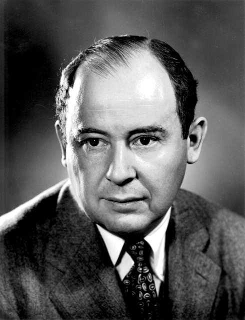
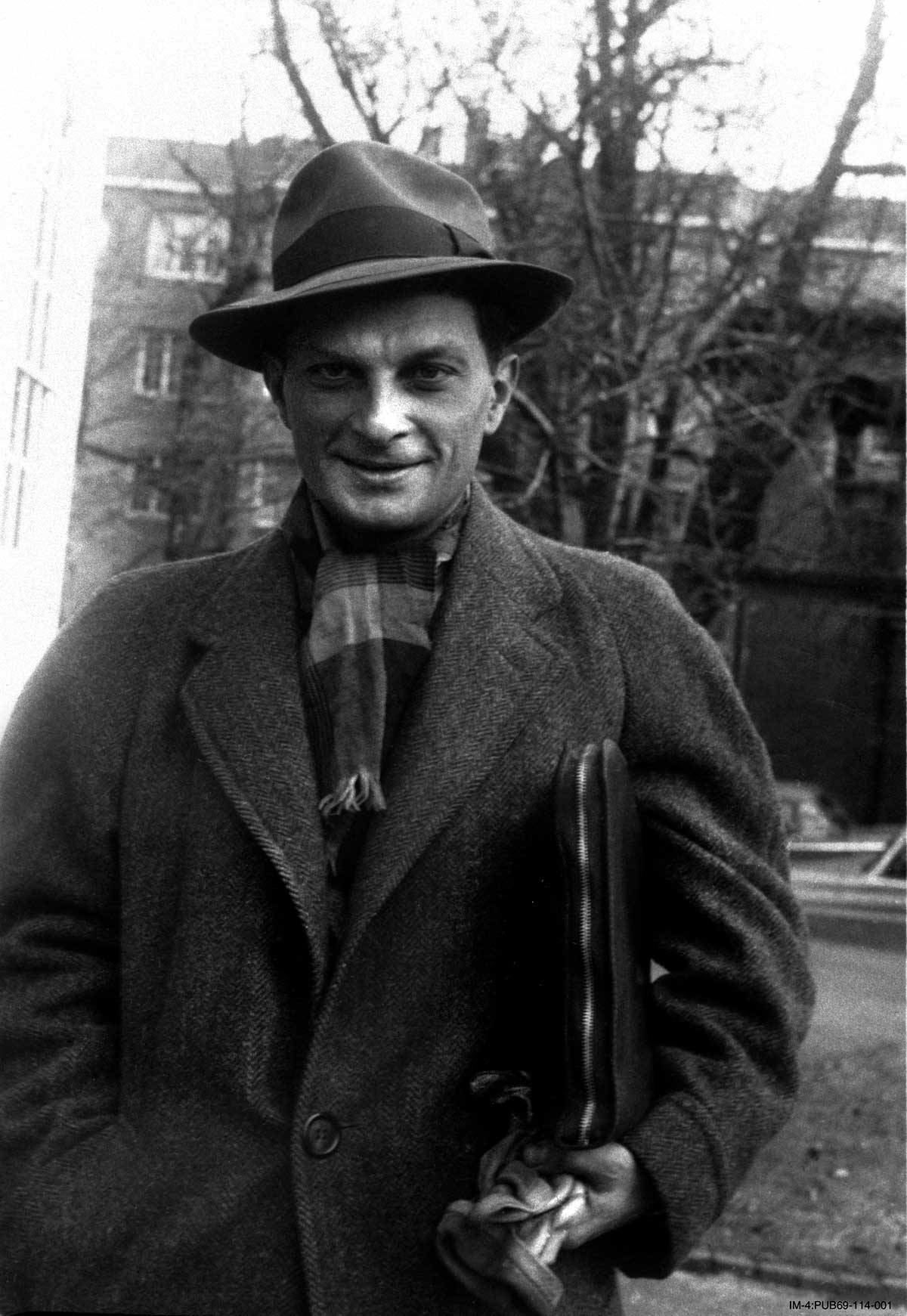
The Russian Roulette estimator was invented by John von Neumann
John von Neumann (1903-1957) was a Hungarian-American mathematician, physicist, computer scientist, engineer and polymath. He's widely regarded as inventing stochastic computing in ². Interestingly, his theory could not be implemented until 10 years later with advances in computing. and Stanislaw Ulam
Stanisław Marcin Ulam (1909 – 1984) was a Polish-American scientist in the fields of mathematics and nuclear physics. He participated in the Manhattan Project, originated the Teller-Ulam design of thermonuclear weapons, discovered the concept of the cellular automaton, invented the Monte Carlo method of computation, and suggested nuclear pulse propulsion. during the 1940s in the context of the Manhattan project.

The name of this estimator comes from the Russian Roulette game of chance, in which a player places a single round in a revolver and shoots at himself. As in the deadly game, the estimator decides through a game of chance whether to continue or stop or continue playing. However, because of the secrecy of the project, they never published it.

The information we have about their discovery is second-hand from colleagues that built upon and credited von Neumann and Ulam them the original discovery. One of the first applications of this technique was to design an unbiased estimator of the matrix pseudoinverse, which we'll discuss in section 3. This application was published by George Forsythe, and the paper starts by crediting Von Neumann and Ulam for the method: The following unusual method of inverting a class of matrices was devised by J. von Neumann and S. M. Ulam.

Since Ulam and von Neumann's discovery, the method has found applications in fields as diverse as computer graphics and particle physics. In machine learning, it has found application in the optimization of recurrent neural netwoks, Bayesian inference, Bayesian nonparametrics, reinforcement learning, and implicit differentiation.

The Russian Roulette Estimator

Consider a sequence $\{Y_1, Y_2, \ldots\}$ with finite limit $Y_{\infty}$. How can we estimate the limit after having seen only a finite number of elements?.

The Russian Roulette is an estimator that allows to do precisely this: estimate the limit of a (potentially infinite) sequence using finite computation, thanks to the magic of randomness.

It works as follows. In the first iterate, the estimator takes the first element in the sequence. Then at each subsequent iteration, the algorithm produces a Bernouilli trial with a probability of success $p$. If the trial was successful, then the algorithm stops and returns the current estimate. If trial was not successful, then the algorithm continues and updates the current estimate $\Yhat$ with a new element of the sequence: $\Yhat + (1-p)^{-t}(Y_t - Y_{t-1})$.

Russian Roulette Estimator
Input: Probability $p \in [0, 1)$, initial estimate $Y_0$
Set $\Yhat = Y_0$
For $t=1, \ldots$ do
With probability $p$: halt and return $\Yhat$
Compute $Y_t$ and $\Yhat = \Yhat + (1-p)^{-t}(Y_t - Y_{t-1})$

Unlike most algorithms, this one doesn't stop after a pre-determined number of iteration. Instead, the number of iterations the algorithm performs –which I'll refer to as the stopping time– is itself a random variable. It's probability is then given by the number of Bernoulli trials needed to get one success. This is the definition of the geometric distribution with parameter $p$.

Showing that $\Yhat$ is an unbiased estimator of the limit can be done by expanding the definition of $\Yhat$ and taking expectations. It's also interesting to note that the elements $Y_i$ in the sequence can also be stochastic themselves, and the proofs below goes through as long as the randomness in this sequence is independent of the halting time.

The Russian Roulette is an unbiased estimator estimator of the limit of the sequence. That is, if $\EE$ denotes the expectation with respect to the randomness of the halting time, then we have $\EE[\Yhat] = Y_{\infty}$.

Let $T$ denote the total number of iterations performed by the estimator $\Yhat$ and ${\color{brown}\unicode{x1D7D9}_{\{i \lt T\}}}$ denote a variable that is $1$ if $i \lt T$ and $0$ otherwise (throughout the blog post I'll use color to highlight quantities that are random). Using this notation, we can write the Russian roulette as the infinite sum \begin{equation}\label{eq:russian_roulette_infinite} \Yhat = Y_0 + {\textstyle\sum_{i=1}^{\infty}} {\color{brown}\unicode{x1D7D9}_{\{i \lt T\}}}(1-p)^{-i} (Y_i - Y_{i-1}) \,, \end{equation} as all terms after $T$ will be zero. Since we know that $T$ follows a geometric distribution with parameter $p$, we can use this to compute $ \EE[{\color{brown}\unicode{x1D7D9}_{\{i \lt t\}}}]=\Proba(i \lt t) = 1 - \Proba(t \leq i)$. This last term is the cumulative distribution function of a geometric distribution, which is $1 - (1-p)^i$, and so $\EE[{\color{brown}\unicode{x1D7D9}_{\{i \lt t\}}}] = (1-p)^{i}$. Finally, taking expectations in the above formula and using this last fact we have the desired unbiasedness: \begin{align} \EE\big[\Yhat\big] &=\EE\left[Y_0 + {\textstyle\sum_{i=1}^{\infty}} {\color{brown}\unicode{x1D7D9}_{\{i \lt T\}}}(1-p)^{-i} (Y_i - Y_{i-1}) \right]\\ &= Y_0 + {\textstyle\sum_{i=1}^{\infty}} \EE[{\color{brown}\unicode{x1D7D9}_{\{i \lt T\}}}] (1-p)^{-i} (Y_i - Y_{i-1})\\ &=Y_0 + {\textstyle\sum_{i=1}^{\infty}} (Y_i - Y_{i-1}) = Y_{\infty}\,. \end{align}

Application: Estimator of the Matrix Pseudoinverse

One of the first applications of the Russian Roulette was as an estimator of the pseudo-inverse $A^\dagger$ of a positive semi-definite matrix $A$. This estimator is based on the Neumann series for the matrix pseudo-inverse: \begin{equation} A^{\dagger} = \gamma \sum_{i=0}^\infty (I - \gamma A)^i \,. \end{equation} This series is known to converge for any $\gamma \lt 2 / \lambda_{\max}$, where $\lambda_{\max}$ is $A$'s largest eigenvalue. We'll assume $\gamma$ is chosen such that the series is convergent.

We can then take as the items in the Russian Roulette sequence the partial sums of the above series, that is, $Y_t \defas \gamma \sum_{i=0}^t (I - \gamma A)^i $. This way, in light of the above identity, the pseudo-inverse is given by the limit $\lim_{t \to \infty}Y_t$. In this case, it will be more convenient to store the difference between two consecutive elements $\Delta_t \defas Y_{t} - Y_{t-1} = \gamma (I - \gamma A)^{t} = \Delta_{t-1} - \gamma A \Delta_{t-1}$, rather than the elements in the sequence $Y_0, Y_1, \ldots$. The resulting algorithm is:

Matrix Pseudoinverse Estimator
Input: Probability $p \in [0, 1)$
Set $\Yhat = \Delta_0 = \gamma I$
For $t=1, \ldots$ do
With probability $p$: halt and return $\Yhat$
Update $\Delta_{t} = \Delta_{t-1} - \gamma A \Delta_{t-1}$
Update $\Yhat = \Yhat + (1-p)^{-t}\Delta_t$

If only an estimator of $A^\dagger b$ is necessary for some vector $b$, the above algorithm can be adapted by replacing the initialization with $\Yhat = X_0 = \gamma b$. This algorithm then doesn't need to store any matrices, only vectors.

This is amazing! How come it's not more widely used?

Exactly my thought after learning about this estimator! However, after having used it in different problems, my initial enthusiasm soon vanished. The Russian Roulette comes with severe drawbacks.

While unbiasedness is a desirable property, it's not the only thing that matters. A controlled variance is another key ingredient of a good estimator. For example, an estimator with infinite variance has infinite mean squared error no law of large numbers. It's hard to see how such an estimator would be useful. And it turns out that the Russian Roulette, unless one is extremely careful, will lead to an estimator with infinite variance.

Let's then take a look at the variance of the Russian Roulette.I'll call variance the quantity $\EE[\|\Yhat - Y_{\infty}\|_F^2]$, where $\|X\|^2_F = \tr(X^\top X)$ is the Frobenius norm. This corresponds to the classical variance when $Y_i$ is a scalar, but is also well defined for matrix and vector-valued estimators. Some authors refers to this as the generalized variance. The following lemma computes the variance of this estimator.

I believe this result is new, or at least I haven't been able to find it in the literature. The closest I found is ¹² who discusses issues relative to the variance of this and other estimators, but they don't provide a simple formula like this one. If you disagree, please leave a comment! The variance of the Russian Roulette estimate is \begin{equation}\label{eq:variance} \EE[\|\Yhat - Y_{\infty}\|_F^2] = \underbrace{\sum_{i=0}^{\infty}p\,\left({{1-p}}\right)^{-(i+1)}}_{\text{diverging}} \underbrace{\vphantom{\sum_{i=0}^{\infty}}\|Y_i - Y_{\infty}\|_F^2}_{\text{converging}} \,. \end{equation}

Show proof

The proof is rather straightforward once the error $Y_{\infty} - \Yhat$ is written as a sum of $R_i \defas Y_i - Y_{\infty}, R_{-1} = 0$ terms. Since $R_i - R_{i-1} = Y_i - Y_{i-1}$ we can write the Russian Roulette estimator from \eqref{eq:russian_roulette_infinite} as $\Yhat = Y_0 + \sum_{i=1}^\infty{\color{brown}\unicode{x1D7D9}_{\{i \lt T\}}} (1-p)^{-i}(R_{i} - R_{i-1})$. Subtracting $Y_{\infty}$ and taking norms we then have \begin{align} \|Y_{\infty} - \Yhat\|^2 &= \|\sum_{i=0}^\infty{\color{brown}\unicode{x1D7D9}_{\{i \lt T\}}} (1-p)^{-i}(R_{i} - R_{i-1})\|^2\\ &= \|\sum_{i=0}^{\infty} \underbrace{({\color{brown}\unicode{x1D7D9}_{\{i+1 \lt T\}}}(1-p)^{-(i+1)} - {\color{brown}\unicode{x1D7D9}_{\{i \lt T\}}}(1-p)^{-i})}_{\defas {\color{olive}q_i} } R_i\|^2 \\ & = \sum_{i=0}^\infty {\color{olive}q_i}^2 \|R_i\|^2 + 2 \sum_{i=1}^{\infty} \sum_{j=i+1}^{\infty} {\color{olive}q_i} {\color{olive}q_j} \tr(R_i^\top R_j)\,. \end{align}

The variance of our estimator is the expectation of the above expression, and so will depend on the expectations of ${\color{olive}q_i}^2$ and ${\color{olive}q_i} {\color{olive}q_j}$. Let's take a closer look at these quantities. The first one can be easily computed by expanding the square and noticing that ${\color{brown}\unicode{x1D7D9}_{\{i+1 \lt T\}}}{\color{brown}\unicode{x1D7D9}_{\{i \lt T\}}} = {\color{brown}\unicode{x1D7D9}_{\{i+1 \lt T\}}}$: \begin{align} \EE[{\color{olive}q_i}^2] &= \EE[{\color{brown}\unicode{x1D7D9}_{\{i+1 \lt T\}}}](1-p)^{-2 (i+1)} + \EE[{\color{brown}\unicode{x1D7D9}_{\{i \lt T\}}}](1-p)^{-2i} - 2 \overbrace{\EE[{\color{brown}\unicode{x1D7D9}_{\{i+1 \lt T\}}}{\color{brown}\unicode{x1D7D9}_{\{i \lt T\}}}]}^{\EE[{\color{brown}\unicode{x1D7D9}_{\{i+1 \lt T\}}}] = (1-p)^{-(i+1)}}(1-p)^{-2i - 1}] \\ &= (1-p)^{-(i+1)} - (1-p)^{-i}\\ &= p (1-p)^{-(i+1)}\,. \end{align} If $i \lt j$ we have ${\color{brown}\unicode{x1D7D9}_{\{i \lt T\}}}{\color{brown}\unicode{x1D7D9}_{\{j \lt T\}}} = {\color{brown}\unicode{x1D7D9}_{\{j \lt T\}}}$ and ${\color{brown}\unicode{x1D7D9}_{\{i +1 \lt T\}}}{\color{brown}\unicode{x1D7D9}_{\{j \lt T\}}} = {\color{brown}\unicode{x1D7D9}_{\{j \lt T\}}}$. We can use this to simplify the expectation of the cross product: \begin{align} \EE\left[{\color{olive}q_i} {\color{olive}q_j} \,|\, i\lt j\right] &= \EE ({\color{brown}\unicode{x1D7D9}_{\{j+1 \lt T\}}}(1-p)^{-(j+1)} - {\color{brown}\unicode{x1D7D9}_{\{j \lt T\}}}(1-p)^{-j})({\color{brown}\unicode{x1D7D9}_{\{i+1 \lt T\}}}(1-p)^{-(i+1)} - {\color{brown}\unicode{x1D7D9}_{\{i \lt T\}}}(1-p)^{-i})\\ &= \underbrace{\EE {\color{brown}\unicode{x1D7D9}_{\{j+1 \lt T\}}} (1-p)^{-(j+1)}}_{=1}\left[ (1-p)^{- (i+1)} - (1-p)^{ - i}\right] - \underbrace{\EE{\color{brown} \unicode{x1D7D9}_{\{j \lt T\}}}(1-p)^{-j}}_{=1}\left[ (1-p)^{-(i+1)} - (1-p)^{-i}\right]\\ &= 0\,. \end{align} Finally, taking expectations on the error norm we have \begin{align} \EE \|Y_{\infty} - \Yhat\|^2 & = \sum_{i=0}^\infty \overbrace{\EE[{\color{olive}q_i}^2]}^{=p(1-p)^{-(i+1)}} \|R_i\|^2 + 2 \sum_{i=1}^{\infty} \sum_{j=i+1}^{\infty} \overbrace{\EE[{\color{olive}q_i} {\color{olive}q_j}]}^{=0} \tr(R_i^\top R_j)\\ &= \sum_{i=0}^\infty p(1-p)^{-(i+1)} \|R_i\|^2 \,, \end{align} and the Theorem statement follows by definition of $R_i$.

Let's unpack what this means. The variance expression above contains the infinite geometric series $\sum_{i=0}^{\infty}p\,\left({{1-p}}\right)^{-(i+1)}$. Since the ratio of this series $(1-p)^{-1}$ is always greater than $1$ for any $p > 0$, this series is diverging. For the infinite sum (and so the variance) to be bounded, it's necessary that the terms $\|Y_{\infty} - Y_i\|^2_F$ multiplying this series compensate this divergence. Although we've assumed $Y_t$ converges to $Y_{\infty}$ as $t \to \infty$ and so these terms asymptotically vanish, this is not enough for the variance to be finite. For the variance to be finite, it's that the ratio of series \eqref{eq:variance} is smaller than one. In other words, the terms $\|Y_{\infty} - Y_i\|^2_F$ need to converge at a speed faster than $\mathcal{O}((1-p)^t)$.

That's a lot to ask. For example, in the example of the matrix pseudoinverse, it's known that Neumann series with step-size $\gamma=\frac{1}{\lambda_{\max}}$ converges with the rate $\|Y_{\infty} - Y_i\|_F = \mathcal{O}\big((1 - \frac{\lambda_{\min}}{\lambda_{\max}})^{2t}\big)$. This gives the very narrow set acceptable values for $p$, namely $p \leq \frac{\lambda_{\min}}{\lambda_{\max}}(2 - \frac{\lambda_{\min}}{\lambda_{\max}})$.This bound could be improved to $p \leq \sqrt{\frac{\lambda_{\min}}{\lambda_{\max}}}(2 - \sqrt{\frac{\lambda_{\min}}{\lambda_{\max}}})$ by using the Chebyshev approximation to the inverse instead of the Neumann series. Although with a slightly better dependency, the average number of iterations $1/p$ will blow up as the inverse condition number $\frac{\lambda_{\min}}{\lambda_{\max}}$ vanishes. For problems with $\frac{\lambda_{\min}}{\lambda_{\max}} = 0.01$ (which is a relatively well-conditioned problem, practical problems often have an inverse condition number of $10^{-6}$), this gives the very narrow set of acceptable values $p \lt 0.0199$ (which results in estimators with an average number of iterations $\geq 50$). And it only gets worse as the problems becomes more ill-conditioned!

Take-home message

The Russian Roulette will often result in useless estimators with infinite variance. Unless one is extremely careful and chooses fast-converging sequences or large average number of iterations (small $p$), then the variance of this estimator will be infinite.

Conclusion

The Russian Roulette is an unbiased estimator for the limit of a sequence. Its applications seem endless, as many hard problems can be cast as estimating the limit of a sequence. This includes –but not limited to– inverting a matrix, minimizing a function, computing recurrent computational graphs or performing bayesian inference.

However, my initial enthusiasm soon turned into skepticism. From the variance analysis, we found out that the range of cases where the Russian Roulette leads to a useful estimator is very narrow.

This might explain the fact that –to the best of my knowledge– none of the methods based on the Russian Roulette described in the application section have become mainstream.

Finally, I'd like to mention that this is not the only unbiased estimator of the limit. There are other ones with potentially better properties, which I haven't discussed in this blog post. For example (Beatson et al. 2019), discusses the alternative single-sample estimator.

Acknowledgements

Thanks to Charles Sutton, Mark Girolami, James Harrison and Charline Le Lan for discussions around this topic and feedback on the blog post.

Citing

If you find this blog post useful, please consider citing as

The Russian Roulette: An Unbiased Estimator of the Limit, Fabian Pedregosa, 2022

with bibtex entry:


  @misc{pedregosa2022russian,
    title={The Russian Roulette: An Unbiased Estimator of the Limit},
    author={Fabian Pedregosa},
    howpublished = {\url{http://fa.bianp.net/blog/2022/russian-roulette/}},
    year={2022}
  }

Keep the gradient flowing