TL; DR These are some notes on calibration of surrogate loss functions in the context of machine learning. But mostly it is an excuse to post some images I made.

In the binary-class classification setting we are given $n$ training samples $\{(X_1, Y_1), \ldots, (X_n, Y_n)\}$, where $X_i$ belongs to some sample space $\mathcal{X}$, usually $\mathbb{R}^p$ but for the purpose of this post we can keep i abstract, and $y_i \in \{-1, 1\}$ is an integer representing the class label.

We are also given a loss function $\ell: \{-1, 1\} \times \{-1, 1\} \to \mathbb{R}$ that measures the error of a given prediction. The value of the loss function $\ell$ at an arbitrary point $(y, \hat{y})$ is interpreted as the cost incurred by predicting $\hat{y}$ when the true label is $y$. In classification this function is often the zero-one loss, that is, $\ell(y, \hat{y})$ is zero when $y = \hat{y}$ and one otherwise.

The goal is to find a function $h: \mathcal{X} \to [k]$, the classifier, with the smallest expected loss on a new sample. In other words, we seek to find a function $h$ that minimizes the expected $\ell$-risk, given by $$ \mathcal{R}_{\ell}(h) = \mathbb{E}_{X \times Y}[\ell(Y, h(X))] $$

In theory, we could directly minimize the $\ell$-risk and we would have the optimal classifier, also known as Bayes predictor. However, there are several problems associated with this approach. One is that the probability distribution of $X \times Y$ is unknown, thus computing the exact expected value is not feasible. It must be approximated by the empirical risk. Another issue is that this quantity is difficult to optimize because the function $\ell$ is discontinuous. Take for example a problem in which $\mathcal{X} = \mathbb{R}^2, k=2$, and we seek to find the linear function $f(X) = \text{sign}(X w), w \in \mathbb{R}^2$ and that minimizes the $\ell$-risk. As a function of the parameter $w$ this function looks something like

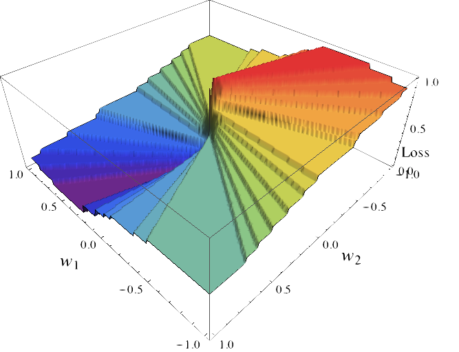
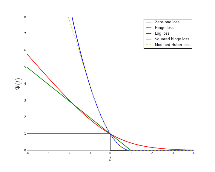
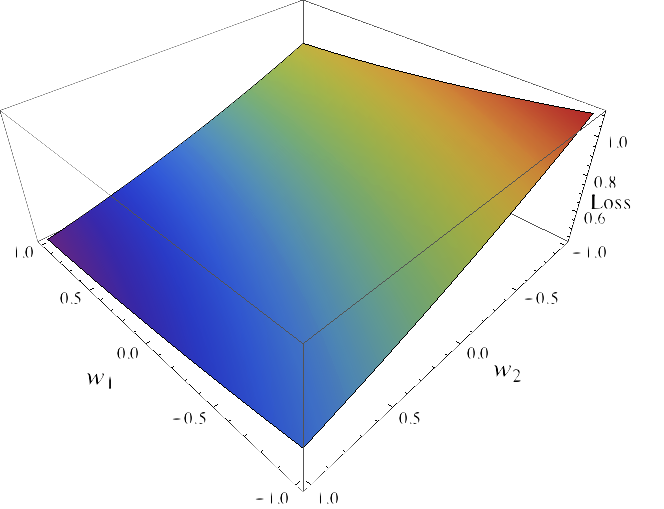
This function is discontinuous with large, flat regions and is thus extremely hard to optimize using gradient-based methods. For this reason it is usual to consider a proxy to the loss called a surrogate loss function. For computational reasons this is usually convex function $\Psi: \mathbb{R} \to \mathbb{R}_+$. An example of such surrogate loss functions is the hinge loss, $\Psi(t) = \max(1-t, 0)$, which is the loss used by Support Vector Machines (SVMs). Another example is the logistic loss, $\Psi(t) = 1/(1 + \exp(-t))$, used by the logistic regression model. If we consider the logistic loss, minimizing the $\Psi$-risk, given by $\mathbb{E}_{X \times Y}[\Psi(Y, f(X))]$, of the function $f(X) = X w$ becomes a much more more tractable optimization problem:

In short, we have replaced the $\ell$-risk which is computationally difficult to optimize with the $\Psi$-risk which has more advantageous properties. A natural questions to ask is how much have we lost by this change. The property of whether minimizing the $\Psi$-risk leads to a function that also minimizes the $\ell$-risk is often referred to as consistency or calibration. For a more formal definition see [¹] and [²]. This property will depend on the surrogate function $\Psi$: for some functions $\Psi$ it will be verified the consistency property and for some not. One of the most useful characterizations was given in [¹] and states that if $\Psi$ is convex then it is consistent if and only if it is differentiable at zero and $\Psi'(0) < 0$. This includes most of the commonly used surrogate loss functions, including hinge, logistic regression and Huber loss functions.