There's a fascinating link between minimization of quadratic functions and polynomials. A link that goes deep and allows to phrase optimization problems in the language of polynomials and vice versa. Using this connection, we can tap into centuries of research in the theory of polynomials and shed new light on old problems.

Introduction

This post deals with a connection between optimization algorithms and polynomials. The problem that we will be looking at throughout the post is that of finding a vector $\xx^\star \in \RR^d$ that minimizes the convex quadratic objective \begin{equation}\label{eq:opt} f(\xx) \defas \frac{1}{2}\xx^\top \HH \xx + \bb^\top \xx~, \end{equation} where $\HH$ is a symmetric positive definite matrix.The quadratic assumption is made for the purpose of the analysis. All the discussed algorithms are applicable to any smooth (not necessarily quadratic) function.

A popular class of algorithms for this problem are gradient-based methods. These are methods in which the next iterate is a linear combination of the previous iterate and past gradients. In the next section we will see how we can identify any gradient-based method with a polynomial that determines the method's convergence speed. And vice-versa, we will see in section 3 that it's possible to do the inverse path and go from a (subset of) polynomials to optimization methods. Then we will use this connection to derive the Chebyshev iterative method, which forms the basis of some of the most used optimization methods such as Polyak momentum, which will be the topic of the next blog post.

Pioneers of Scientific Computing

The ideas outlined in this post can be traced back to the early years of numerical analysis. Minimizing quadratic objective functions (or equivalently solving linear systems of equations) was one of the first applications of scientific computing, and while some methods like gradient descent (Cauchy, 1847) and Gauss-Seidel predate the development of electronic computers, their algorithmic analysis as we know it today emerged during the 1940s and 1950s.

One of the first applications of the theory of polynomials to the solution of linear systems is the development of the Chebyshev iterative method, done independently by Flanders and Shortley, Cornelius Lanczos, and David Young, and further analyzed and popularized by Richard Varga and Gene Golub. Shortly after the development of the Chebyshev iterative method, the field saw one of the most beautiful applications of the theory of orthogonal polynomials in numerical analysis, the conjugate gradient method.

An excellent review on the topic is the 1959 book chapter “Theory of Gradient Methods” by H. Rutishauser,
Heinz Rutishauser (1918–1970). Among other contributions, he introduced a number of basic syntactic features to programming, notably the keyword "for" for a for loop, first as the German "für" in Superplan, next via its English translation "for" in ALGOL 58A. which has stood remarkably well the test of time. A more modern but equally excellent review is the 1996 book by Bernd Fisher.

These ideas are still relevant today. Just in the last year, these tools have been used for example to develop accelerated decentralized algorithms, to derive lower bounds and to develop methods that are optimal for the average-case.

From Optimization to Polynomials

In this section we will develop a method to assign to every optimization method a polynomial that determines its convergence. We will first motivate this approach through gradient descent and then generalize it to other methods.

Motivation: Gradient Descent

Consider the gradient descent method that generates iterates following \begin{equation} \xx_{t+1} = \xx_t - \tfrac{2}{L + \lmin} \nabla f(\xx_t)~, \end{equation} where $L$ and $\lmin$ are the largest and smallest eigenvalue of $\HH$ respectively. Our goal is to derive a bound on the error $\|\xx_{t+1} - \xx^\star\|$ as a function of the number of iterations $t$ and the spectral properties of $\HH$.

By the first order optimality conditions, at the optimum we have $\nabla f(\xx^\star) = 0$ and so $\HH \xx^\star = - \bb$ by the quadratic assumption. We can use this to write the gradient as $\nabla f(\xx_t) = \HH (\xx_t - \xx^\star)$. Subtracting $\xx^\star$ from both sides of the above equation we have \begin{align} &\xx_{t+1} - \xx^\star = \xx_t - \tfrac{2}{L + \lmin} \HH (\xx_t - \xx^\star) - \xx^\star\\ &\quad= (\II - \tfrac{2}{L + \lmin} \HH)(\xx_t - \xx^\star)\\ &\quad= (\II - \tfrac{2}{L + \lmin} \HH)^2(\xx_{t-1} - \xx^\star) = \cdots \\ &\quad= (\II - \tfrac{2}{L + \lmin} \HH)^{t+1} (\xx_0 - \xx^\star) \end{align} We now have an expression for $\xx_{t+1} - \xx^\star$ in terms of the initial conditions $\xx_0 - \xx^\star$, and a polynomial of degree $t$ in $\HH$. Taking the 2-norm on both sides and using Cauchy-Schwartz we have \begin{align} \|\xx_{t+1} - \xx^\star\|_2 &\leq \|(\II - \tfrac{2}{L + \lmin}\HH)^{t+1}\|_2 \|\xx_0 - \xx^\star\|_2\label{eq:gd_cauchy_schwartz}\\ &\leq \max_{\lambda \in [\lmin, L]}\, |(1 - \tfrac{2}{L + \lmin} \lambda)^{t+1}| \|\xx_0 - \xx^\star\|_2 \label{eq:gd_respol_bound} \end{align} where the second inequality follows by the definition matrix 2-norm of a symmetric matrix. In this bound, convergence is determined by the maximum absolute value of the polynomial \begin{equation} P^{\text{GD}}_{t+1} \defas \left(1 - \tfrac{2}{L + \lmin} \lambda\right)^{t+1}~. \end{equation} Here's a plot of this polynomial, together with its maximum absolute value represented with a dashed line:

The residual polynomial for gradient descent, $P_t(\lambda) = (1 - 2 \lambda / (\lmax + \lmin))$. Only even degrees are displayed for visualization purposes.

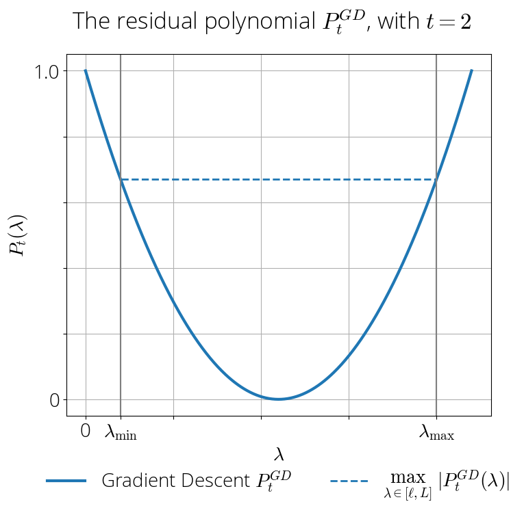
As expected, as $t$ increases, the polynomial goes to zero in the interval $[\lmin, L]$. Furthermore, the largest absolute value of the polynomial is achieved at the edges, and we can use this to bound its maximum value in \eqref{eq:gd_respol_bound}. This leads to the following classical bound on the error: \begin{equation} \|\xx_t - \xx^\star\| \leq \left(\frac{\lmax - \lmin}{\lmax + \lmin} \right)^{t}\|\xx_0 - \xx^\star\|~. \end{equation}

Generalization to Gradient-based Methods

We will now show how the previous approach generalizes to any gradient-based method. These are methods where the update is a linear combination of the current iterate, current gradient and difference of previous iterates \begin{equation}\label{eq:gradient_based} \xx_{t+1} = \xx_{t} + \sum_{i=0}^{t-1} c^{(t)}_{i} (\xx_{i+1}\!-\!\xx_{i}) + c^{(t)}_{t} \nabla f(\xx_{t})~, \end{equation} for some scalar values $c^{(t)}_{j}$.This is a large class of methods that include gradient descent, (Nesterov) momentum but not methods with matrix preconditioners like BFGS since the coefficients are required to be scalars. To this method, we will associate the following residual polynomial $P_t$, which is a polynomial of degree $t$ defined recursively as \begin{equation} \begin{split} P_{t+1}(\lambda) &= (1 + c^{(t)}_{t} \lambda)P_{t}(\lambda) + \sum_{i=0}^{t-1} c^{(t)}_{i}(P_{i+1}(\lambda)\!-\!P_{i}(\lambda))\\ P_0(\lambda) &= 1~. \end{split}\label{eq:def_residual_polynomial} \end{equation}

By construction, all residual polynomials verify $P_t(0) = 1$.

The following lemma shows how the residual polynomial can be useful in the analysis of optimization methods. In particular, it shows how to express the error ($\xx_t - \xx^\star$) in terms of the residual polynomial:It's rare in optimization to have an exact expression for the complexity of an algorithm, and not just a potentially loose upper bound. This is one of those cases.

For any gradient-based method and any iteration $t$, we have \begin{equation} \xx_t - \xx^\star = P_t(\HH)(\xx_0 - \xx^\star) \label{eq:residual_error}~. \end{equation}

Given its simplicity, it's easy to glance upon this lemma, so let's take a minute to appreciate its significance. It says that for any gradient-based method I can express the error $\xx_t - \xx^\star$ exactly as a product of two terms. One term is the error at initialization $\xx_0 - \xx^\star$ and doesn't depend on the optimization method. The other term instead, $P_t(\HH)$, doesn't depend on the initialization but does depend on the optimization method. Since we only have control over the optimization method, this lemma is telling us that the efficiency of any optimization method can be studied exclusively in terms of its associated residual polynomial $P_t$.

From this lemma we can also derive a bound that replaces the matrix polynomial by a scalar bound, which is often more interpretable. For this, consider the eigendecomposition of $\HH = \QQ \LLambda \QQ^T$, where $\QQ$ is orthonormal and $\LLambda$ is a diagonal matrix with diagonal elements the eigenvalues of $\HH$. Then taking norms in \eqref{eq:residual_error} and using this decomposition we have \begin{align} \|\xx_t - \xx^\star\| &= \|P_t(\HH) (\xx_0 - \xx^\star)\|\\ &\leq \|P_t(\HH)\|\|\xx_0 - \xx^\star\|\quad \text{ (Cauchy-Schwartz)}\\ &= \|P_t(\LLambda)\|\|\xx_0 - \xx^\star\| \quad \text{ (eigendecomposition)} \end{align} Finally, since $P_t(\LLambda)$ is a diagonal matrix, its operator norm is given by its largest element. This leads to the following bound:

Let $\lmin$ and $L$ be the smallest and largest eigenvalue of $\HH$ respectively. Then for any gradient-based method with residual polynomial $P_t$, we have \begin{equation} \|\xx_t - \xx^\star\| \leq {\color{purple}\underbrace{\max_{\lambda \in [\lmin, L] }}_{\text{conditioning}}} \, {\color{teal}\underbrace{\vphantom{\max_{[L]}}|P_t(\lambda)|}_{\text{algorithm}} } \,\, {\color{brown}\underbrace{\vphantom{\max_{[L]}}\|\xx_0 - \xx^\star\|}_{\text{initialization}}}~. \end{equation}

This Corollary will be very useful in the following as it constructs a bound on the distance to optimum based on the three aspects that most influence convergence:

• The algorithm enters this bound through its residual polynomial. The smaller image of the residual polynomial, the better. Of course, we have the constraint $P_t(0) = 1$, which makes choosing this polynomial non-trivial.
• The conditioning of the problem enters through the eigenvalue interval $[\lmin, L]$.
• The initialization enters through its distance to optimum.

Of the quantities in the above lemma, $\max_{\lambda \in [\lmin, L]} |P_t(\lambda)|$ is an upper bound on the progress that the algorithm makes at iteration $t$. This quantity will be useful in the following to compare the convergence properties of different algorithm. We will refer to it as the (worst-case) convergence rate of a method.

All the convergence rates in this post are worst-case bounds. By this I mean that the bounds hold for any problem within a class (quadratic problems of the form \eqref{eq:opt} in this post). However, for certain problems the empirical convergence often is better than the theoretical bound. Furthermore, these bounds don't say anything about the typical performance of a method, which is more representative of the actual performance of a method. In a recent work, Damien and I explored the average-case complexity of optimization algorithms, first in the non-asymptotic regime and then in the asymptotic one. The average-case analysis of optimization algorithms will be the subject of a future post.

Optimal Residual Polynomial

In the previous section we've seen that the convergence rate of gradient descent is $\left(\frac{\lmax - \lmin}{\lmax + \lmin} \right)^{t}$. Is this the optimal convergence rate or can we do better?

To answer these questions we will use a somewhat indirect approach. Instead of seeking directly the optimal method, we will instead seek the optimal residual polynomial, and then reverse-engineer the method from its polynomial. This technique turns out to be more appropriate since it will allow us to use powerful results from the polynomial approximation literature.

By optimal in this case I mean the polynomial with smallest convergence rate $\max_{\lambda \in [\lmin, L]}|P(\lambda)|$. This corresponds to solving the following problem over the space of polynomials \begin{equation} \argmin_{P}\max_{\lambda \in [\lmin, L]}|P(\lambda)|~, \end{equation} where the minimization is over all degree $t$ residual polynomials. The normalization $P(0) = 1$ of residual polynomials makes this problem non-trivial, as otherwise the optimal solution would be $P(\lambda) = 0$.

The residual polynomial that minimizes the above expression turns out to be intimately related to Chebyshev polynomials, which are one of the most used families of polynomials in numerical analysis.
Chebyshev polynomials bear the name of Pafnuty Chebyshev (1821-1894). He is considered to be a founding father of Russian mathematics and made important contributions to the fields of probability (Chebyshev inequality), statistics, mechanics and number theory (Bertrand-Chebyshev theorem) among other.

The Chebyshev polynomials of the first kind $T_0, T_1, \ldots$ are defined by the recurrence relation \begin{align} &T_0(\lambda) = 1 \qquad T_1(\lambda) = \lambda\\ &T_{k+1}(\lambda) = 2 \lambda T_k(\lambda) - T_{k-1}(\lambda)~. \end{align}

Among the many properties of Chebyshev polynomials is that a shifted and normalized version of it achieves the optimal convergence rate. Most best polynomial approximation results assume the polynomials are defined in the interval $[-1, 1]$. However, in our case it's more natural to focus on the interval $[\lmin, L]$ that contains the Hessian eigenvalues. To account for this discrepancy, we'll use the following affine mapping \begin{equation} \sigma(\lambda) = \frac{L+\lmin}{L-\lmin} - \frac{2}{L - \lmin}\lambda\,, \end{equation} that maps the interval $[\lmin, L]$ onto $[-1, 1]$ with $\sigma(\lmin) = 1$ and $\sigma(L) = -1$.

We can now introduce a theorem that relates the convergence rate optimality to Chebyshev polynomials. It was first proven by Vladimir Markov Vladimir Markov was a student of Chebyshev and brother of the famous Andrey Markov. Vladimir died of tuberculosis when he was only 25 year old. and later rediscovered by Flanders and Shortley.

The following shifted Chebyshev polynomial has smallest maximum absolute value through the interval $[\lmin, \lmax]$ (where $\lmin > 0$) among all residual polynomials of degree $t$: \begin{equation}\label{eq:def_residual_chebyshev} P^{\text{cheb}}_t(\lambda) \defas \frac{T_t(\sigma(\lambda))}{T_t(\sigma(0))}~. \end{equation} We will refer to this polynomial as the residual Chebyshev polynomial.

As we did for gradient descent, I find it interesting to visualize the residual polynomials. Below is the Chebyshev and gradient descent residual polynomial, together with their maximum absolute value ($\equiv$convergence rate) shown in dashed lines.

Gradient descent and Chebyshev residual polynomials

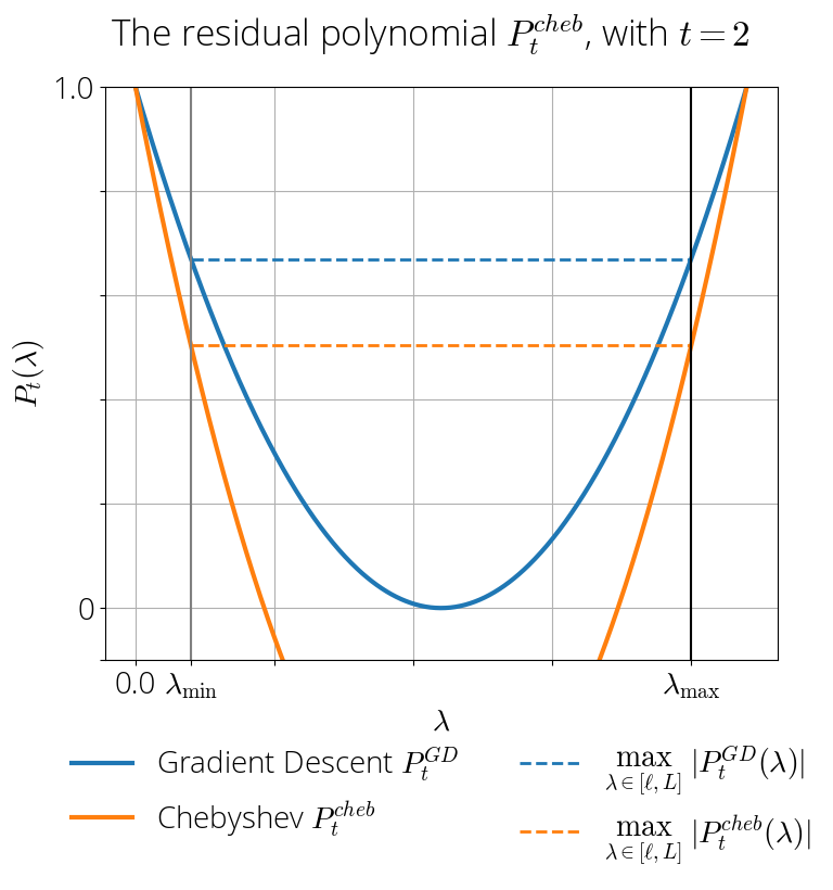
As expected from the theory, the maximum of the Chebyshev polynomial (dashed orange line) is significatively smaller than that of the gradient descent residual polynomial, which translates into a faster convergence rate. We can also see from this plot that the Chebyshev residual polynomial, unlike gradient descent, reaches its extremal value not just once in the edges, but $t+1$ times, a fact that was crucial argument in proving Markov's Theorem.

The Chebyshev iterative method

From the previous theorem we know that the Chebyshev residual polynomials are optimal in terms of their worst-case convergence rate. We will now derive the method associated with this polynomial. We will do this by deriving the recurrence of the residual polynomial, and then using the definition of residual polynomial to match the method's coefficients.

Let $a = \sigma(0), b = \sigma(\lambda)$. Then using the three term recurrence of the Chebyshev polynomials we have \begin{align} P^{\text{cheb}}_{t+1}(\lambda) &= \frac{T_{t+1}(b)}{T_{t+1}(a)} = 2 b \frac{T_t(b)}{T_{t+1}(a)} - \frac{T_{t-1}(b)}{T_{t+1}(a)}\\ &= 2 b \frac{T_t(a)}{T_{t+1}(a)} P^{\text{cheb}}_t(\lambda) - \frac{T_{t-1}(a)}{T_{t+1}(a)} P^{\text{cheb}}_{t-1}(\lambda)~, \end{align} where in the second identity we have multiplied and divided the first term by $T_t(a)$ and the second term by $T_{t-1}(a)$

Now let $\omega_{t} \defas 2 a\frac{T_t(a)}{ T_{t+1}(a)}$. Then we can rewrite the previous equation as \begin{equation} P^{\text{cheb}}_{t+1}(\lambda) = \omega_t \frac{b}{a} P^{\text{cheb}}_t(\lambda) - \frac{1}{4 a^2} \omega_t \omega_{t-1} P^{\text{cheb}}_{t-1}(\lambda)\,. \end{equation} We would now like to have a cheap way to compute $\omega_t$. Using again the three term recurrence of Chebyshev polynomials on $\omega_{t+1}^{-1}$ we have \begin{align} \omega_{t}^{-1} &= \frac{T_{t+1}(a)}{2 a T_{t}(a)} = \frac{2 a T_t(a) - T_{t-1}(a)}{2 a T_{t}(a)} = 1 - \frac{\omega_{t-1}}{4 a^2} \end{align} and so the full recursion for the residual polynomial becomes \begin{align} &P_0(\lambda) = 1\,,~P_1(\lambda) = 1 - \tfrac{2}{L + \lmin}\lambda\,\\ &\omega_{t} = \left(1 - \tfrac{1}{4 a^2}\omega_{t-1} \right)^{-1} \quad \text{ (with $\omega_0 = 2$)}\\ &P^{\text{cheb}}_{t+1}(\lambda) = \omega_{t} \tfrac{b}{a} P^{\text{cheb}}_t(\lambda) - \tfrac{1}{4 a^2} \omega_{t} \omega_{t-1} P^{\text{cheb}}_{t-1}(\lambda) \end{align} where $\omega_0 = 2$ is computed from the definition of Chebyshev polynomials, $\omega_{0} = 2a T_{0}(a) / T_1(a) = 2 a 1 / a = 2$.

This gives a recurrence for the residual polynomial. We can then use the connection between optimization methods and residual polynomials \eqref{eq:def_residual_polynomial}, this time in reverse, to find the coefficients of the optimization method from its residual polynomial. Matching terms in $P_t$ in the previous equation we have \begin{equation} 1 + \lambda c^{(t)}_{t} + c^{(t)}_{t-1} = \omega_{t}\tfrac{b}{a} = \omega_{t}(1 - \tfrac{2}{L + \lmin}\lambda) \end{equation} and so matching terms in $\lambda$ we get \begin{equation} c^{(t)}_{t} = - \tfrac{2}{L+\lmin} \omega_{t} \qquad c^{(t)}_{t-1} = \omega_{t} - 1~. \end{equation} Replacing these parameters in the definition of a gradient-based method, we obtain the Chebyshev iterative method:

Chebyshev Iterative Method
Input: starting guess $\xx_0$, $\rho = \frac{L - \lmin}{L + \lmin}$, $\omega_{0} = 2$
$\xx_1 = \xx_0 - \frac{2}{L + \lmin} \nabla f(\xx_0)$
For $t=1, 2, \ldots~$ do \begin{align} \omega_{t} &= (1 - \tfrac{\rho^2}{4}\omega_{t-1})^{-1}\label{eq:recurrence_momentum}\\ \xx_{t+1} &= \vphantom{\sum^n}\xx_t + \left(\omega_{t} - 1\right)(\xx_{t} - \xx_{t-1})\nonumber\\ &\quad - \omega_{t}\tfrac{2}{L + \lmin}\nabla f(\xx_t) \end{align}

Although we initially considered a class of methods that can use all previous iterates, the optimal method only requires to store the last iterate and the difference vector $\xx_{t-1} - \xx_{t}$. This makes the method much more practical than if we had to store all previous gradients.

Convergence rate

By construction, the Chebyshev iterative method has an optimal worst-case convergence rate. But what is this optimal rate?

Since the maximum absolute value of the Chebyshev polynomials in $[-1, 1]$ is 1, the convergence rate for $P^{\text{cheb}}$ in this case is \begin{equation} \max_{\lambda \in [\lmin, L]} |P^{\text{cheb}}_t(\lambda)| = T_t\left(\frac{L + \lmin}{L - \lmin}\right)^{-1}~. \end{equation}

This is however not very helpful if we cannot evaluate the Chebyshev polynomial. Luckily, outside the interval $[-1, 1]$ they do admit the following explicit expression \begin{equation}\label{eq:cheb_explicit} T_t(\lambda) = \frac{1}{2} \big[ \big( \lambda + \sqrt{\lambda^2-1} \big)^t + \big(\lambda – \sqrt{\lambda^2-1}\big)^t \big]\,. \end{equation} Setting $\lambda = \tfrac{L + \lmin}{L - \lmin}$ and using the trivial bound $\lambda > \sqrt{\lambda^2-1}$ we have \begin{align} T_t\left(\tfrac{L+\lmin}{L - \lmin}\right) &\geq \frac{1}{2}\left( \tfrac{L+\lmin}{L - \lmin} + \sqrt{\Big( \tfrac{L+\lmin}{L - \lmin}\Big)^2-1} \right)^t \label{eq:bound_chebyshev}\\ &= \frac{1}{2}\left(\tfrac{L + \lmin + 2 \sqrt{\lmin L}}{L - \lmin} \right)^t \\ &= \frac{1}{2}\left(\tfrac{\sqrt{L} + \sqrt{\lmin}}{\sqrt{L} - \sqrt{\lmin}} \right)^t ~, \end{align} where last identity follows from completing the square in the numerator and using the identity $L - \lmin = (\sqrt{L} - \sqrt{\lmin})(\sqrt{L} + \sqrt{\lmin})$ in the denominator. We have hence computed the convergence rate associated with the Chebyshev residual polynomial:

Let $\xx_1, \xx_2, \ldots$ be the iterates generated by the Chebyshev iterative method. Then we have the following bound \begin{equation} \|\xx_t - \xx^\star\| \leq 2\left( \frac{\sqrt{L} - \sqrt{\lmin}}{\sqrt{L} + \sqrt{\lmin}}\right)^t \|\xx_0 - \xx^\star\| \,. \end{equation}

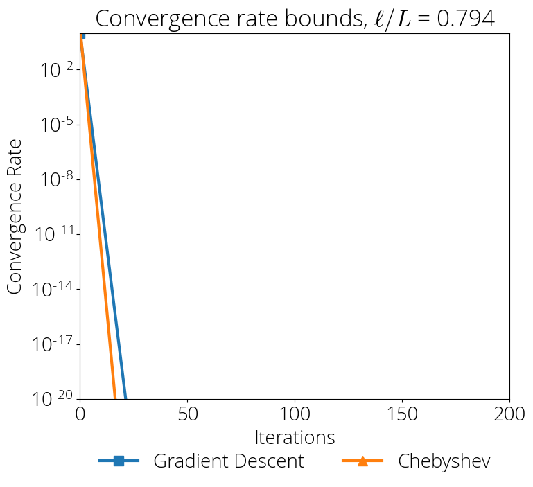
Note that the term $2\left( \frac{\sqrt{L} - \sqrt{\lmin}}{\sqrt{L} + \sqrt{\lmin}}\right)^t$ is not the exact rate $\max_{\lambda \in [\lmin, L]} |P^{\text{cheb}}_t(\lambda)|$ but instead an upper bound on this quantity due to the bound we used in \eqref{eq:bound_chebyshev}. This explains why under some choices of $L$, $\lmin$ and $t$ the rate is worse than that of gradient descent despite being the method with an optimal convergence rate.

Despite the looseness of the bound, we can see that the square root in the $L$ and $\lmin$ constants can in some circumstances make the convergence rate much smaller, specially in cases in which $\lmin$ is much smaller than $L$, which is a common setting, since in machine learning $\lmin$ is often very close to zero. Below is a comparison of the convergence rate

Comparison of convergence rates bounds for gradient descent and Chebyshev.

Citing

If you find this blog post useful, please consider citing it as:

Residual Polynomials and the Chebyshev method., Fabian Pedregosa, 2020

Bibtex entry:

  
    @misc{pedregosa2021residual,
      title={Residual Polynomials and the Chebyshev method},
      author={Pedregosa, Fabian},
      howpublished = {\url{http://fa.bianp.net/blog/2020/polyopt/}},
      year={2020}
    }
  
  

Conclusion

In this post we've seen how to assign a polynomial to any gradient-based optimization method, how to use this polynomial to obtain convergence guarantees and how to use it to derive optimal methods. Using this framework we've derived the Chebyshev iterative method.

In the next posts, I will relate Polyak momentum (aka HeavyBall) to this framework.

Thanks to Baptiste Goujaud for detailed feedback and reporting many typos, Damien Scieur —polynomial wizzard and amazing collaborator—, Nicolas Le Roux, Courtney Paquette and Adrien Taylor —for encouragement and stimulating discussions—, Francis Bach —for pointers and great writings on this topic—, Ali Rahimi for feedback on this post, Nicolas Loizou, and Waiss Azizian for discussions.

Updates. [2020/02/06] Reddit discussion.

References