On the Link Between Optimization and Polynomials, Part 3
A Hitchhiker's Guide to Momentum.
I've seen things you people wouldn't believe.
Valleys sculpted by trigonometric functions.
Rates on fire off the shoulder of divergence.
Beams glitter in the dark near the Polyak gate.
All those landscapes will be lost in time, like tears in rain.
Time to halt.
A momentum optimizer *
Gradient Descent with Momentum
Gradient descent with momentum,
Gradient Descent with Momentum
Input: starting guess $\xx_0$, step-size $\step > 0$ and momentum
parameter $\mom \in (0, 1)$.
$\xx_1 = \xx_0 - \dfrac{\step}{\mom+1} \nabla f(\xx_0)$
For $t=1, 2, \ldots$ compute
\begin{equation}\label{eq:momentum_update}
\xx_{t+1} = \xx_t + \mom(\xx_{t} - \xx_{t-1}) - \step\nabla
f(\xx_t)
\end{equation}
Despite its simplicity, gradient descent with momentum exhibits unexpectedly rich dynamics that we'll explore on this post.
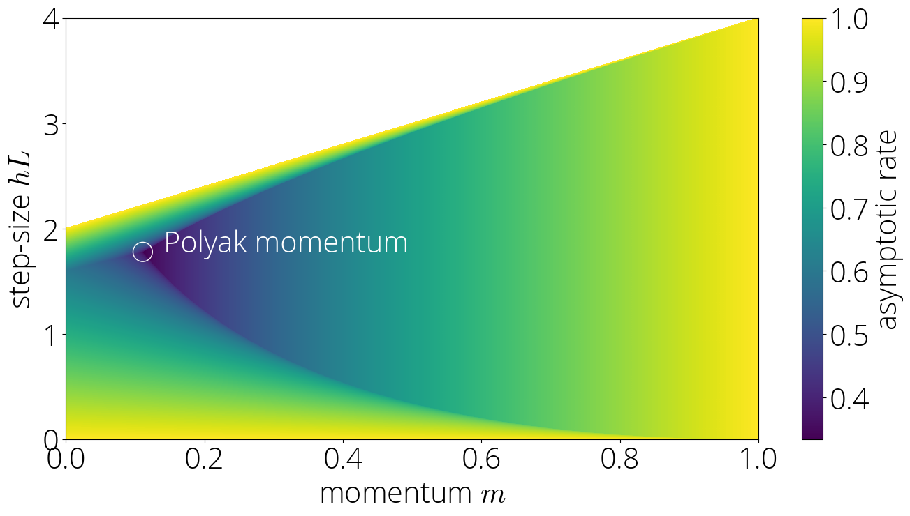
The landscape described in the section "The Dynamics of Momentum" are different than the ones described in this post. The ones in Gabriel's paper describe the improvement along the direction of a single eigenvector, and as such are at best a partial view of convergence (in fact, they give the misleading impression that the best convergence is achieved with zero momentum). The techniques used in this post allow instead to compute the global convergence rate, and figures like the above correctly predict a non-trivial optimal momentum term.
Convergence rates
In the last post we saw that, assuming $f$ is a quadratic objective of the form \begin{equation}\label{eq:opt} f(\xx) \defas \frac{1}{2}\xx^\top \HH \xx + \bb^\top \xx~, \end{equation} then we can analyze gradient descent with momentum using a convex combination of Chebyshev polynomials of the first and second kind.
More precisely, we showed that the error at iteration $t$ can be bounded as \begin{equation}\label{eq:theorem} \|\xx_t - \xx^\star\| \leq \underbrace{\max_{\lambda \in [\lmin, L]} |P_t(\lambda)|}_{\defas r_t} \|\xx_0 - \xx^\star\|\,.\\ \end{equation} where $\lmin$ and $L$ are the smallest and largest eigenvalues of $\HH$ respectively and $P_t$ is a $t$-th degree polynomial that we can write as \begin{align} P_t(\lambda) = \mom^{t/2} \left( {\small\frac{2\mom}{1+\mom}}\, T_t(\sigma(\lambda)) + {\small\frac{1 - \mom}{1 + \mom}}\,U_t(\sigma(\lambda))\right)\,. \end{align} where $\sigma(\lambda) = {\small\dfrac{1}{2\sqrt{\mom}}}(1 + \mom - \step\,\lambda)\,$ is a linear function that we'll refer to as the link function and $T_t$ and $U_t$ are the Chebyshev polynomials of the first and second kind respectively.
We'll denote by $r_t$ the maximum of this polynomial over the $[\lmin, L]$ interval, and call the convergence rate of an algorithm the $t$-th root of this quantity, $\sqrt[t]{r_t}$. We'll also use often the limit superior of this quantity, $\limsup_{t \to \infty} \sqrt[t]{r_t}$, which we'll call the asymptotic rate. The asymptotic rate provides a convenient way to compare the (asymptotic) speed of convergence, as it allows to ignore other slower terms that are negligible for large $t$.
This identity between gradient descent with momentum and Chebyshev polynomials opens the door to deriving the asymptotic properties of the optimizer from those of Chebyshev polynomials.
The Two Faces of Chebyshev Polynomials
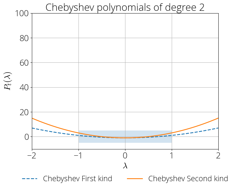
Chebyshev polynomials behave very differently inside and outside the interval $[-1, 1]$. Inside this interval (shaded blue region) the magnitude of these polynomials stays close to zero, while outside it explodes:
Let's make this observation more precise.
Inside the $[-1, 1]$ interval, Chebyshev polynomials admit the trigonometric definitions $T_t(\cos(\theta)) = \cos(t \theta)$ and $U_{t}(\cos(\theta)) = \sin((t+1)\theta) / \sin(\theta)$ and so they have an oscillatory behavior with values bounded in absolute value by 1 and $t+1$ respectively.
Outside of this interval the Chebyshev polynomials of the first kind admit the explicit form for $|\xi| \ge 1$:
\begin{align}
T_t(\xi) &= \dfrac{1}{2} \Big(\xi-\sqrt{\xi^2-1} \Big)^t + \dfrac{1}{2} \Big(\xi+\sqrt{\xi^2-1} \Big)^t \\
U_t(\xi) &= \frac{(\xi + \sqrt{\xi^2 - 1})^{t+1} - (\xi - \sqrt{\xi^2 - 1})^{t+1}}{2 \sqrt{\xi^2 - 1}}\,.
\end{align}
We're interested in convergence rates, so we'll look into $t$-th root asymptotics of the quantities.
The Robust Region
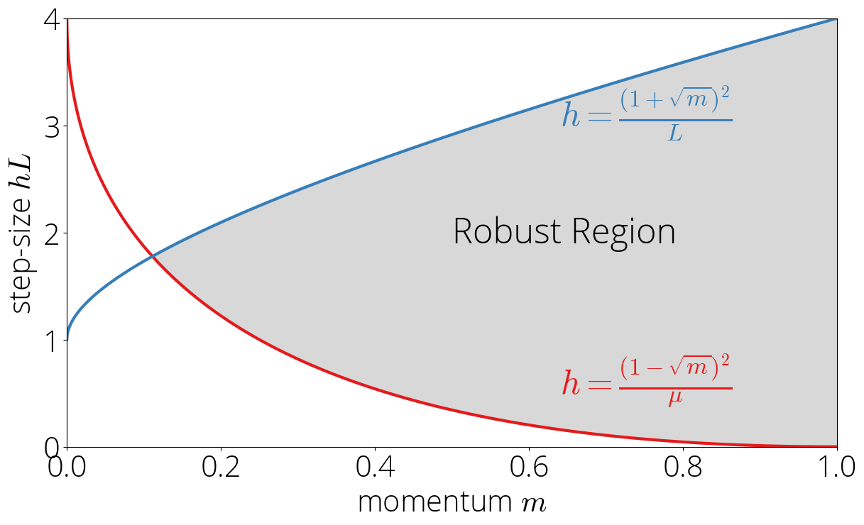
Let's start first by considering the case in which the Chebyshev polynomials are only evaluated in the $[-1, 1]$. Since the Chebsyshev polynomials are evaluated at $\sigma(\cdot)$, this implies that $|\sigma(\lambda)| \leq 1$. We'll call the set of step-size and momentum parameters for which the previous inequality is verified the robust region.
Let's visualize this region in a map. Since $\sigma$ is a linear function, its extremal values are reached at the edges: \begin{equation} \max_{\lambda \in [\lmin, L]} |\sigma(\lambda)| = \max\{|\sigma(\lmin)|, |\sigma(L)|\}\,. \end{equation} Using $\lmin \leq L$ and that $\sigma(\lambda)$ is decreasing in $\lambda$, we can simplify the condition that the above is smaller than one to $\sigma(\lmin) \leq 1$ and $\sigma(L) \geq -1$, which in terms of the step-size and momentum correspond to: \begin{equation}\label{eq:robust_region} \frac{(1 - \sqrt{\mom})^2}{\lmin} \leq \step \leq \frac{(1 + \sqrt{\mom})^2}{L} \,. \end{equation} These two conditions provide the upper and lower bound of the robust region.
Asymptotic rate
Let $\sigma(\lambda) = \cos(\theta)$ for some $\theta$, which is always possible since $\sigma(\lambda) \in [-1, 1]$. In this regime, Chebyshev polynomials verify the identities $T_t(\cos(\theta)) = \cos(t \theta)$ and $U_t(\cos(\theta)) = \sin((t+1)\theta)/\sin(\theta)$ , which replacing in the definition of the residual polynomial gives \begin{equation} P_t(\sigma^{-1}(\cos(\theta))) = \mom^{t/2} \left[ {\small\frac{2\mom}{1+\mom}}\, \cos(t\theta) + {\small\frac{1 - \mom}{1 + \mom}}\,\frac{\sin((t+1)\theta)}{\sin(\theta)}\right]\,. \end{equation}
Since the expression inside the square brackets is bounded in absolute value by $t+2$, taking $t$-th root and then limits we have $\limsup_{t \to \infty} \sqrt[t]{|P_t(\sigma^{-1}(\cos(\theta)))|} = \sqrt{\mom}$ for any $\theta$. This gives our first asymptotic rate:
The asymptotic rate in the robust region is $\sqrt{\mom}$.
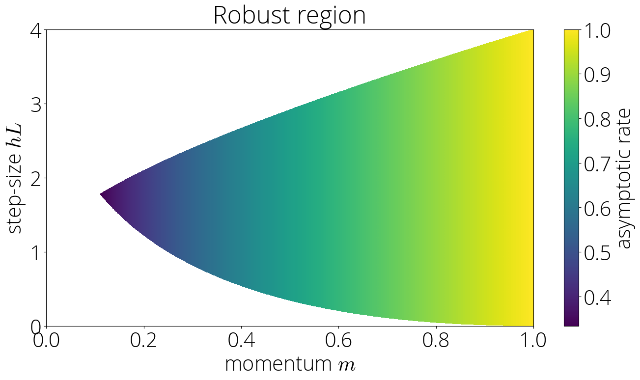
This is nothing short of magical. It would seem natural –and this will be the case in other regions– that the speed of convergence should depend on both the step-size and the momentum parameter. Yet, this result implies that it's not the case in the robust region. In this region, the convergence only depends on the momentum parameter $\mom$. Amazing.
This also illustrates why we call this the robust region. In its interior, perturbing the step-size in a way that we stay within the region has no effect on the convergence rate. The next figure displays the asymptotic rate (darker is faster) in the robust region.
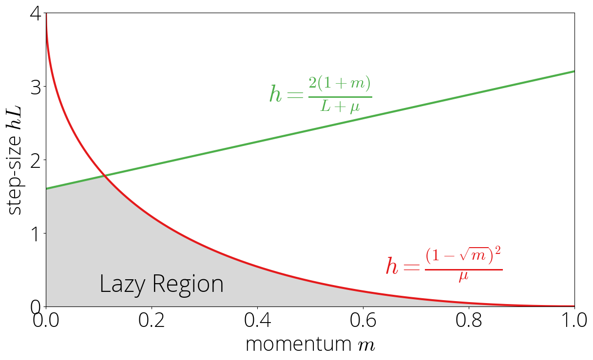
The Lazy Region
Let's consider now what happens outside of the robust region. In this case, the convergence will depend on the largest of $\{|\sigma(\lmin)|, |\sigma(L)|\}$. We'll consider first the case in which the maximum is $|\sigma(\lmin)|$ and leave the other one for next section.
This region is determined by the inequalities $|\sigma(\lmin)| > 1$ and $|\sigma(\lmin)| \geq |\sigma(L)|$. Using the definition of $\sigma$ and solving for $\step$ gives the equivalent conditions \begin{equation} \step \leq \frac{2(1 + \mom)}{L + \lmin} \quad \text{ and }\quad \step \leq \frac{(1 - \sqrt{\mom})^2}{\lmin}\,. \end{equation} Note the second inequality is the same one as for the robust region \eqref{eq:robust_region} but with the inequality sign reversed, and so the region will be on the oposite side of that curve. We'll call this the lazy region, as in increasing the momentum will take us out of it and into the robust region.
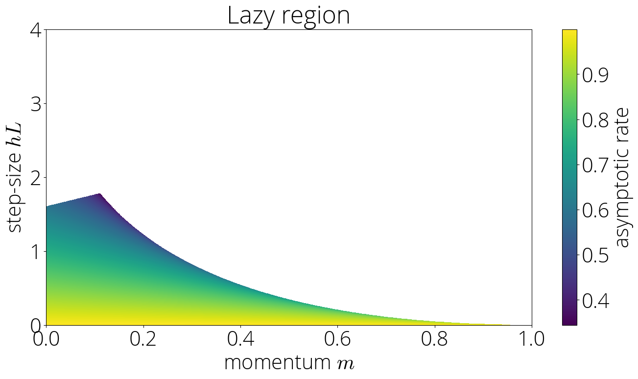
Asymptotic rate
As we saw in Section 2, outside of the $[-1, 1]$ interval both Chebyshev have simple $t$-th root asymptotics. Using this and that both kinds of Chebyshev polynomials agree in sign outside of the $[-1, 1]$ interval we can compute the asymptotic rate as \begin{align} \lim_{t \to \infty} \sqrt[t]{r_t} &= \sqrt{\mom} \lim_{t \to \infty} \sqrt[t]{ {\small\frac{2\mom}{\mom+1}}\, T_t(\sigma(\lmin)) + {\small\frac{1 - \mom}{1 + \mom}}\,U_t(\sigma(\lmin))} \\ &= \sqrt{\mom}\left(|\sigma(\lmin)| + \sqrt{\sigma(\lmin)^2 - 1} \right)\\ \end{align} This gives the asymptotic rate for this region
In the lazy region the asymptotic rate is $\sqrt{\mom}\left(|\sigma(\lmin)| + \sqrt{\sigma(\lmin)^2 - 1} \right)$.
Unlike in the robust region, this rate depends on both the step-size and the momentum parameter, which enters in the rate through the link function $\sigma$. This can be observed in the color plot of the asymptotic rate
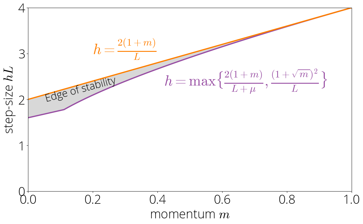
Edge of Stability
The robust and lazy region occupy most (but not all!) of the region for which momentum converges. There's a small region that sits between the lazy and robust regions and the region where momentum diverges. We call this region the edge of stability
For parameters not in the robust or lazy region, we have that $|\sigma(L)| > 1$ and $|\sigma(L)| > |\sigma(\lmin)|$. Using the asymptotics of Chebyshev polynomials as we did in the previous section, we have that the asymptotic rate is $\sqrt{\mom}\left(|\sigma(L)| + \sqrt{\sigma(L)^2 - 1} \right)$. The method will only converge when this asymptotic rate is below 1. Enforcing this results in $\step \lt 2 (1 + \mom) / L$. Combining this condition with the one of not being in the robust or lazy region gives the characterization: \begin{equation} \step \lt \frac{2 (1 + \mom)}{L} \quad \text{ and } \quad \step \geq \max\Big\{\tfrac{2(1 + \mom)}{L + \lmin}, \tfrac{(1 + \sqrt{\mom})^2}{L}\Big\}\,. \end{equation}
Asymptotic rate
The asymptotic rate can be computed using the same technique as in the lazy region. The resulting rate is the same as in that region but with $\sigma(L)$ replacing $\sigma(\lmin)$:
In the Knife's edge region the asymptotic rate is $\sqrt{\mom}\left(|\sigma(L)| + \sqrt{\sigma(L)^2 - 1} \right)$.
Pictorially, this corresponds to

Putting it all together
This is the end of our journey. We've visited all the regions on which momentum converges.
The asymptotic rate $\limsup_{t \to \infty} \sqrt[t]{r_t}$ of momentum is \begin{alignat}{2} &\sqrt{\mom} &&\text{ if }\step \in \big[\frac{(1 - \sqrt{\mom})^2}{\lmin}, \frac{(1+\sqrt{\mom})^2}{L}\big]\\ &\sqrt{\mom}(|\sigma(\lmin)| + \sqrt{\sigma(\lmin)^2 - 1}) &&\text{ if } \step \in \big[0, \min\{\tfrac{2(1 + \mom)}{L + \lmin}, \tfrac{(1 - \sqrt{\mom})^2}{\lmin}\}\big]\\ &\sqrt{\mom}(|\sigma(L)| + \sqrt{\sigma(L)^2 - 1})&&\text{ if } \step \in \big[\max\big\{\tfrac{2(1 + \mom)}{L + \lmin}, \tfrac{(1 + \sqrt{\mom})^2}{L}\big\}, \tfrac{2 (1 + \mom) }{L} \big)\\ &\geq 1 \text{ (divergence)} && \text{ otherwise.} \end{alignat}
Plotting the asymptotic rates for all regions we can see that Polyak momentum (the method with momentum $\mom = \left(\frac{\sqrt{L} - \sqrt{\lmin}}{\sqrt{L} + \sqrt{\lmin}}\right)^2$ and step-size $\step = \left(\frac{2}{\sqrt{L} + \sqrt{\lmin}}\right)^2$ which is asymptotically optimal among the momentum methods with constant coefficients) is at the intersection of the three regions.
![]()
Citing
If you find this blog post useful, please consider citing it as:
A Hitchhiker's Guide to Momentum, Fabian Pedregosa, 2021
Bibtex entry:
    @misc{pedregosa2021residual,
      title={A Hitchhiker's Guide to Momentum},
      author={Pedregosa, Fabian},
      howpublished = {\url{http://fa.bianp.net/blog/2021/hitchhiker/}},
      year={2021}
    }
Acknowledgements. Thanks to Baptiste Goujaud for proofreading, catching many typos and making excellent clarifying suggestions, to Robert Gower for proofreading this post and providing thoughtful feedback. Thanks also to Courtney Paquette and Adrien Taylor for reporting errors.