Backtracking step-size strategies (also known as adaptive step-size or approximate line-search) that set the step-size based on a sufficient decrease condition are the standard way to set the step-size on gradient descent and quasi-Newton methods. However, these techniques are much less common for Frank-Wolfe-like algorithms. In this blog post I discuss a backtracking line-search for the Frank-Wolfe algorithm.

info This is the third post in a series on the Frank-Wolfe algorithm. See here for Part 1, Part 2.

Introduction

The Frank-Wolfe (FW) or conditional gradient algorithm is a method for constrained optimization that solves problems of the form

\begin{equation}\label{eq:fw_objective} \minimize_{\xx \in \mathcal{D}} f(\boldsymbol{x})~, \end{equation}

where $f$ is a smooth function for which we have access to its gradient and $\mathcal{D}$ is a compact set. We also assume to have access to a linear minimization oracle over $\mathcal{D}$, that is, a routine that solves problems of the form \begin{equation} \label{eq:lmo} \ss_t \in \argmax_{\boldsymbol{s} \in \mathcal{D}} \langle -\nabla f(\boldsymbol{x}_t), \boldsymbol{s}\rangle~. \end{equation}

From an initial guess $\xx_0 \in \mathcal{D}$, the FW algorithm generates a sequence of iterates $\xx_1, \xx_2, \ldots$ that converge towards the solution to \eqref{eq:fw_objective}.

Frank-Wolfe algorithm
Input: initial guess $\xx_0$, tolerance $\delta > 0$
$\textbf{For }t=0, 1, \ldots \textbf{ do } $
    $\boldsymbol{s}_t \in \argmax_{\boldsymbol{s} \in \mathcal{D}} \langle -\nabla f(\boldsymbol{x}_t), \boldsymbol{s}\rangle$
    Set $\dd_t = \ss_t - \xx_t$ and $g_t = \langle - \nabla f(\xx_t), \dd_t\rangle$
    Choose step-size ${\stepsize}_t$ (to be discussed later)
    $\boldsymbol{x}_{t+1} = \boldsymbol{x}_t + {\stepsize}_t \dd_t~.$
$\textbf{end For loop}$
$\textbf{return } \xx_t$

As other gradient-based methods, the FW algorithm depends on a step-size parameter ${\stepsize}_t$. Typical choices for this step-size are:

1. Predefined decreasing sequence. The simplest choice, developed in (Dunn and Harshbarger 1978) and more recently popularized in (Clarkson 2010, Jaggi 2013)^,, is to choose the step-size according to the pre-defined decreasing sequence \begin{equation} {\stepsize}_t = \frac{2}{t+2}~. \end{equation} This choice of step-size is straightforward and cheap to compute. However, in practice it performs worst than the alternatives, although it enjoys the same worst-case complexity bounds.

2. Exact line-search. Another alternative is to take the step-size that maximizes the decrease in objective along the update direction: \begin{equation}\label{eq:exact_ls} \stepsize_\star \in \argmin_{\stepsize \in [0, 1]} f(\xx_t + \stepsize \dd_t)~. \end{equation} By definition, this step-size gives the highest decrease per iteration. However, solving \eqref{eq:exact_ls} can be a costly optimization problem, so this variant is not practical except on a few specific cases where the above problem is easy to solve (for instance, in quadratic objective functions).

3. Demyanov-Rubinov step-size. A less-known but highly effective step-size strategy for FW in the case in which we have access to the Lipschitz constant of $\nabla f$, denoted $\Lipschitz$,$\nabla f$ is $L$-Lipschitz if $\|\nabla f(\xx) - \nabla f(\yy)\| \leq \Lipschitz \|\xx - \yy\|$ for all $\xx, \yy$ in the domain. is the following: \begin{equation} \label{eq:ls_demyanov} \stepsize = \min\left\{ \frac{g_t}{\Lipschitz\|\dd_t\|^2}, 1\right\}~. \end{equation} Note this step-size naturally goes to zero as we approach the optimum, which as we'll see in the next section is a desirable property. This is because the step-size is proportional to the Frank-Wolfe gap $g_t$, which is a measure of problem suboptimality. This strategy was first published by Demyanov and Rubinov in the 1960s,
Alexander Rubinov (1940 – 2006) (left) and Vladimir Demyanov (1938–) (right) are two Russian pioneers fo optimization. They wrote the optimization textbook Approximate Methods in Optimization Problems, which contains a throughout discussion of the different step-size choices in the Frank-Wolfe algorithm. although surprisingly it seems to be less popular than the other approaches.

Why not backtracking line-search?

Those familiar with methods based on gradient descent might be surprised by the omission of adaptive step-size methods (also known as backtracking line search) from the previous list. In backtracking line-search, the step-size is selected based on a local condition. Examples of these are the Armijo and Goldstein (sometimes collectively referred to as Wolfe) conditions. These strategies have been wildly successful and are a core part of any state-of-the-art implementation of (proximal) gradient descent and Quasi-Newton methods. Surprisingly, backtracking line search have been almost absent from the literature on Frank-Wolfe.

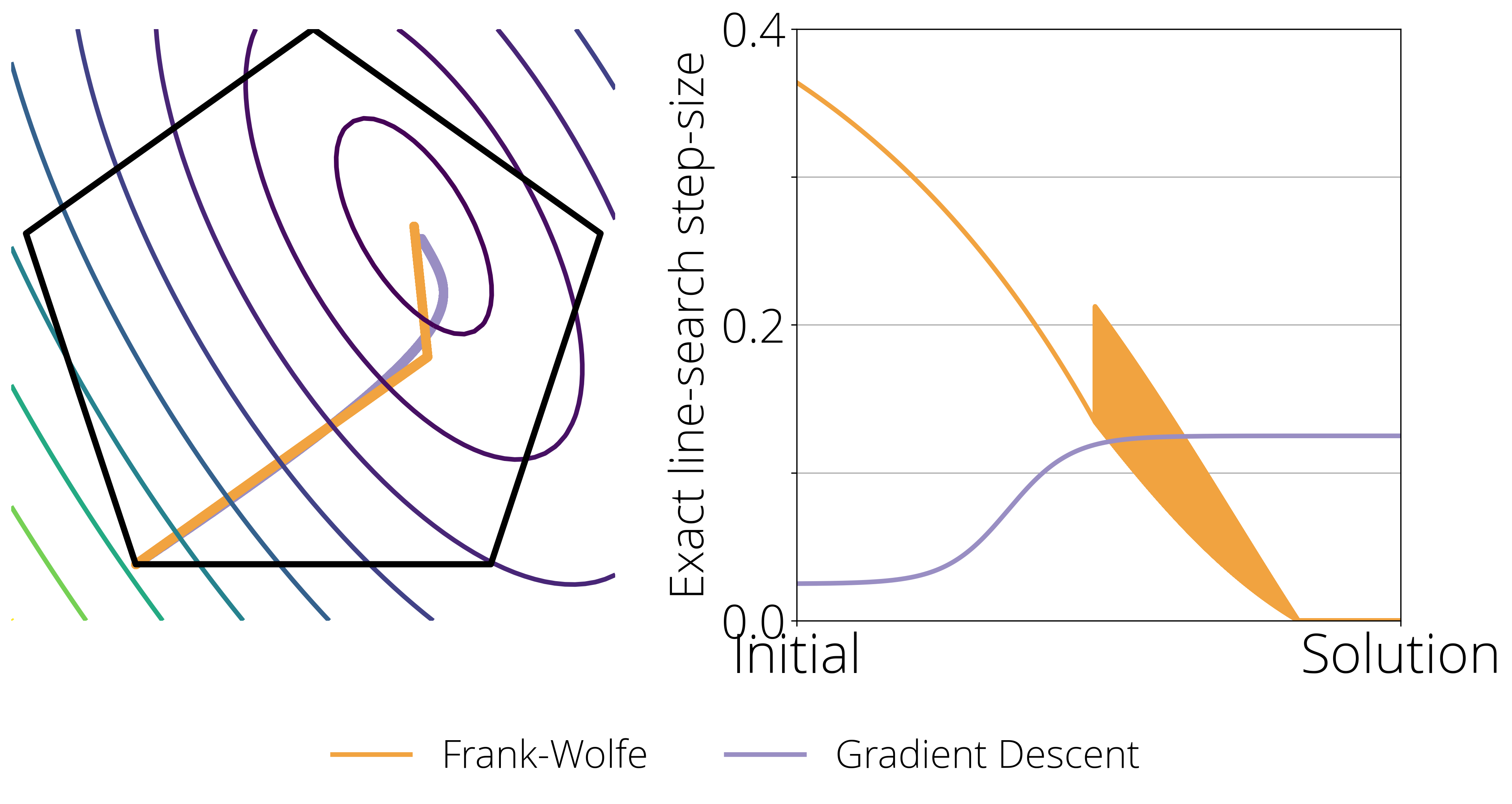
There are important differences between the step-size of FW and gradient descent that can explain this disparity. Consider the following figure. In the left hand side we show a toy 2-dimensional constrained problem, where the level curves represent the value of the objective function, the pentagon are the constrain set, and the orange and violet curve shows the path taken by Frank-Wolfe and Gradient descent respectively when the step-size goes to zero (left). The right side plot shows the optimal step-size (determined by exact line-search) at every point of the optimization path.

This last plot highlights two crucial differences between the Frank-Wolfe and Gradient Descent that we need to keep in mind when designing a step-size scheduler:

• Stability and convergence to zero. Gradient Descent converges with a constant (non-zero) step-size, Frank-Wolfe doesn't. It requires a decreasing step-size to anneal the (potentially non-zero) magnitude of the update.
• Zig-zagging. When close to the optimum, the Frank-Wolfe algorithm often exhibits a zig-zagging behavior, where the selected vertex $d_t$ in the update oscillates between two vertices. The best step-size might be different in these two directions, and so a good strategy should be able to quickly alternate between two different step-sizes.

Dissecting the Demyanov-Rubinov step-size

Understanding the Demyanov-Rubinov step-size will be crucial to developing an effective adaptive step-size in the next section.

The Demyanov-Rubinov step-size can be derived from a quadratic upper bound on the objective. It's a classical result in optimization that a function with $\Lipschitz$-Lipschitz gradient admits the following quadratic upper bound for some constant $\Lipschitz$ and all $\xx, \yy$ in the domain: \begin{equation}\label{eq:l_lsmooth} f(\yy) \leq f(\xx) + \langle \nabla f(\xx), \yy - \xx \rangle + \frac{\Lipschitz}{2}\|\xx - \yy\|^2~. \end{equation} Applying this inequality at the current and next FW iterate $(\xx = \xx_t, \yy = \xx_{t} + \stepsize \dd_t)$ we obtain \begin{equation}\label{eq:l_smooth2} f(\xx_t + \stepsize \dd_t) \leq f(\xx_t) - \stepsize g_t + \frac{\stepsize^2 \Lipschitz}{2}\|\dd_t\|^2~. \end{equation}

The right hand side is a quadratic function of $\stepsize$. Minimizing it subject to the constraint $\stepsize \in [0, 1]$ –to guarantee the iterates remain the domain – gives the following solution:Exact line-search would correspond to minimizing the left hand side. We're relaxing the exact line-search problem and minimizing an upper bound on our true objective. \begin{equation} \stepsize_t^\text{DR} = \min\left\{ \frac{g_t}{\Lipschitz\|\dd_t\|^2}, 1\right\}\,, \end{equation} which is the DR step-size from Eq. \eqref{eq:ls_demyanov}.

Frank-Wolfe with backtracking line-search

The main drawback of the DR step-size is that it requires knowledge of the Lipschitz constant. This limits its usefulness because, first, it might be costly to compute this constant, and secondly, this constant is a global upper bound on the curvature, leading to suboptimal step-sizes in regions where the local curvature might be much smaller.

But there's a way around this limitation. It's possible estimate a step-size such that it guarantees a certain decrease of the objective without using global constants. The first work to attempt this was (Dunn 1980) who developed an analysis for the Goldstein-Armijo line-search. However, the algorithm that we'll present here is based on a different backtracking line-search algorithm which is more adapted to the Frank-Wolfe algorithm. It first appeared to the best of my knowledge in (Beck et al. 2015) and was later refined and generalized to many other Frank-Wolfe variants by myself and coauthors.

In this algorithm, instead of relying on the quadratic upper bound given by the Lipschitz constant, we construct a local quadratic approximation at $\xx_t$. This quadratic function is analogous to \eqref{eq:l_smooth2}, but where the global Lipschitz constant is replaced by the potentially much smaller local constant $\LocalLipschitz_t$: \begin{equation} Q_t(\stepsize, \LocalLipschitz_t) \defas f(\xx_t) - \stepsize g_t + \frac{\stepsize^2 \LocalLipschitz_t}{2} \|\dd_t\|^2\,. \end{equation} As with the Demyanov-Rubinov step-size, we will choose the step-size that minimizes the approximation on the $[0, 1]$ interval, that is \begin{equation} \stepsize_{t} = \min\left\{ \frac{g_t}{\LocalLipschitz_t\|\dd_t\|^2}, 1\right\}\,. \end{equation} Note that this step-size has a very similar form as the DR step-size, but with $\LocalLipschitz_t$ replacing $\Lipschitz$.

This is all fine and good, so far it seems we've only displaced the problem from estimating $\Lipschitz$ to estimating $\LocalLipschitz_t$. Here is where things turn interesting: there's a way to estimate $\LocalLipschitz_t$, that is both convenient and also gives strong theoretical guarantees.

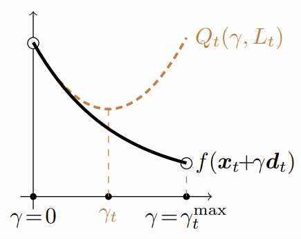
The sufficient decrease condition ensures that the quadratic approximation is an upper bound at its constrained minimum of the line-search objective. For this, we'll choose the $\LocalLipschitz_t$ that makes the quadratic approximation an upper bound at the next iterate: \begin{equation}\label{eq:sufficient_decrease} f(\xx_{t+1}) \leq Q_t(\stepsize_t, \LocalLipschitz_t) \,. \end{equation} This way, we can guarantee that the backtracking line-search step-size makes at least as much progress as exact line-search in the quadratic approximation.

There are many values of $\LocalLipschitz_t$ that verify this condition. For example, from the $\Lipschitz$-smooth inequality \eqref{eq:l_smooth2} we know that any $\LocalLipschitz_t \geq \Lipschitz$ will be a valid choice. However, values of $\LocalLipschitz_t$ that are much smaller than $\Lipschitz$ will be the most interesting, as these will lead to larger step-sizes.

In practice there's little value in spending too much time finding the smallest possible value of $\LocalLipschitz_t$, and the most common strategy consists in initializing this value a bit smaller than the one used in the previous iterate (for example $0.99 \times \LocalLipschitz_{t-1}$), and correct if necessary.

Below is the full Frank-Wolfe algorithm with backtracking line-search. The parts responsible for the estimation of the step-size are between the comments /* begin of backtracking line-search */ and /* end of backtracking line-search */ .

Frank-Wolfe with backtracking line-search
Input: initial guess $\xx_0$, tolerance $\delta > 0$, backtracking line-search parameters $\tau > 1$, $\eta \leq 1$, initial guess for $\LocalLipschitz_{-1}$. Default values for the backtracking parameters that work well in my experience: $\tau = 2.0$ and $\eta = 0.9$. See below for an heuristic on $\LocalLipschitz_{-1}$.
$\textbf{For }t=0, 1, \ldots \textbf{ do } $     $\quad\boldsymbol{s}_t \in \argmax_{\boldsymbol{s} \in \mathcal{D}} \langle -\nabla f(\boldsymbol{x}_t), \boldsymbol{s}\rangle$
    Set $\dd_t = \ss_t - \xx_t$ and $g_t = \langle - \nabla f(\xx_t), \dd_t\rangle$
     /* begin of backtracking line-search */
    $\LocalLipschitz_t = \eta \LocalLipschitz_{t-1}$
    $\stepsize_t = \min\left\{{{g}_t}/{(\LocalLipschitz_t\|\dd_t\|^{2})}, 1\right\}$
    While $f(\xx_t + \stepsize_t \dd_t) > Q_t(\stepsize_t, \LocalLipschitz_t) $ do Increase $\LocalLipschitz_t$ until it satisfies the sufficient decrease condition \eqref{eq:sufficient_decrease}.
        $\LocalLipschitz_t = \tau \LocalLipschitz_t$
     /* end of backtracking line-search */
    $\boldsymbol{x}_{t+1} = \boldsymbol{x}_t + {\stepsize}_t \dd_t~.$
$\textbf{end For loop}$
$\textbf{return } \xx_t$

Let's unpack what happens inside the backtracking line-search block. The block starts by choosing a constant that is a factor of $\eta$ smaller than the one given by the previous iterate. If $\eta = 1$, then it will be exactly the same than the previous iterate, but if $\eta$ is smaller than $1$ (I found $\eta = 0.9$ to be a reasonable default), this will result in a candidate value of $\LocalLipschitz_t$ that is smaller than the one used in the previous iterate. This is done to ensure this constant can decrease if we move to a region with smaller curvature.

In the next line the algorithm sets a tentative value for the step-size based on the formula REF using the current (tentative) value for $\LocalLipschitz_t$. The next line is a While loop that increases $\LocalLipschitz_t$ until it verifies the sufficient decrease condition \eqref{eq:sufficient_decrease}

The algorithm is not fully agnostic to the local Lipschitz constant, as it still requires to set an initial value for this constant, $\LocalLipschitz_{-1}$. One heuristic that I found works well in practice is to initialize it to the (approximate) local curvature along the update direction. For this, select a small $\varepsilon$, say $\varepsilon = 10^{-3}$ and set \begin{equation} \LocalLipschitz_{-1} = \frac{\|\nabla f(\xx_0) - \nabla f(\xx_0 + \varepsilon \dd_0)\|}{\varepsilon \|\dd_0\|}\,. \end{equation}

Convergence rates

By the sufficient decrease condition we have at each iteration \begin{align} \mathcal{P}(\xx_{t+1}) &\leq \mathcal{P}(\xx_t) - \stepsize_t g_t + \frac{\stepsize_t^2 \LocalLipschitz_t}{2}\|\ss_t - \xx_t\|^2 \\ &\leq \mathcal{P}(\xx_t) - \xi_t g_t + \frac{\xi_t^2 \LocalLipschitz_t}{2}\|\ss_t - \xx_t\|^2 \text{ for any $\xi_t \in [0, 1]$} \\ &\leq \mathcal{P}(\xx_t) - \xi_t g_t + \frac{\xi_t^2 \tau \Lipschitz}{2}\|\ss_t - \xx_t\|^2 \text{ for any $\xi_t \in [0, 1]$}\,, \end{align} where in the second inequality we have used the fact that $\stepsize_t$ is the minimizer of this right-hand side over the $[0, 1]$ interval, and so it's an upper bound on any value in this interval. In the third inequality we have used that the sufficient decrease condition is verified for any $\LocalLipschitz \geq \Lipschitz$, and so the backtracking loop cannot bring its value below $\tau \LocalLipschitz$, as long as it was initialized with a value above this constant.

The last identity is the same one we used as starting point in Theorem 3 of the second part of these notes to show the sublinear convergence for convex objectives (with a $\Lipschitz$ instead of $\tau \Lipschitz$). Following the same proof then yields a $\mathcal{O}(\frac{1}{t})$ convergence rate on the primal-dual gap, with $\Lipschitz$ replaced by $\tau \Lipschitz$.

Our paper contains the full proof, including a proof for non-convex objectives, as well as extensions to many other Frank-Wolfe variants such as Pairwise and Away-steps.

Benchmarks

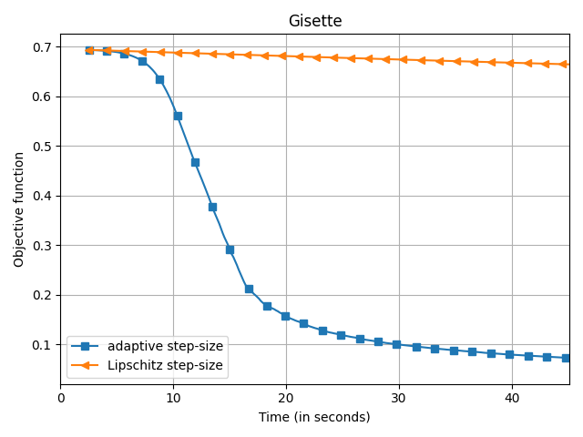
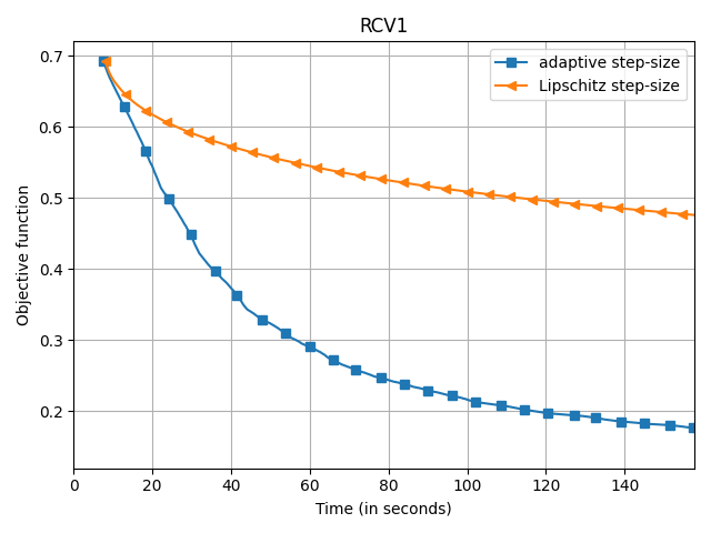
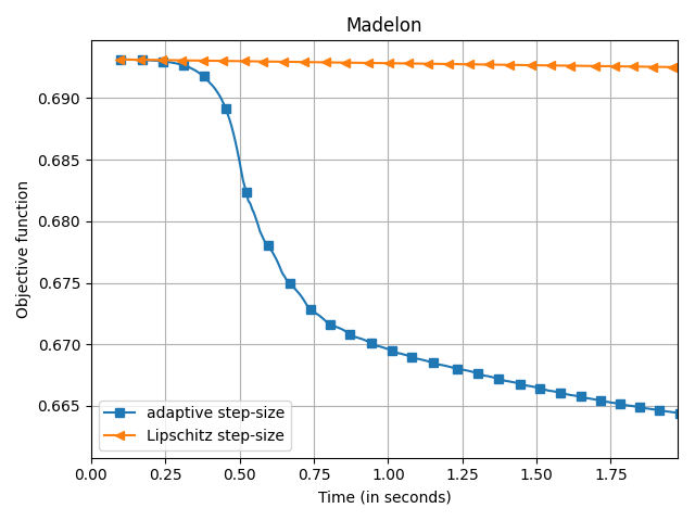
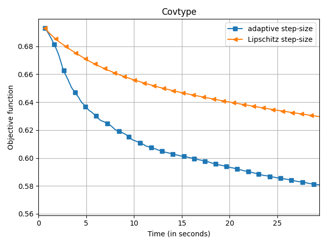
The empirical speedup of the backtracking line-search is huge, sometimes up to an order of magnitude. Below I compare Frank-Wolfe with backtracking line-search (denoted adaptive) and with Demyanov-Rubinov step-size (denoted Lipschitz). All the problems are instances of logistic regression with $\ell_1$ regularization on different datasets using the copt software package.

Citing

If you've found this blog post useful, please consider citing it's full-length companion paper. This paper extends the theory presented here to other Frank-Wolfe variants such as Away-steps Frank-Wolfe and Pairwise Frank-Wolfe. Furthermore, it shows that these variants maintain its linear convergence with backtracking line-search.

Linearly Convergent Frank-Wolfe with Backtracking Line-Search, Fabian Pedregosa, Geoffrey Negiar, Armin Askari, Martin Jaggi. Proceedings of the 22nd International Conference on Artificial Intelligence and Statistics (AISTATS), 2020

Bibtex entry:

  @inproceedings{pedregosa2020linearly,
    title={Linearly Convergent Frank-Wolfe with Backtracking Line-Search},
    author={Pedregosa, Fabian and Negiar, Geoffrey and Askari, Armin and Jaggi, Martin},
    booktitle={International Conference on Artificial Intelligence and Statistics},
    series = {Proceedings of Machine Learning Research},
    year={2020}
  }

Thanks

Thanks Geoffrey Negiar and Quentin Berthet for feedback on this post.

References