I have a dirty secret. Well, I actually have many. But one of them is that I never understood the basic algorithms behind reinforcement learning. So I plan to remedy this in this series of blog posts, where I will cover some of the basic RL algorithms, from REINFORCE to the frontier.

Here's the first one, where I cover one of the oldest practical gradient estimators for reinforcement learning – the REINFORCE estimator – and show how it can get away without differentiating through the environment.

Setup

This is the notation I'll follow throughout the series, which will hopefully be quite standard nowadays. An agent interacts with an environment by observing states $s \in \mathcal{S}$, taking actions $a \in \mathcal{A}$, receiving rewards $r(s, a) \in \RR$, and transitioning to a new state $s'$ according to the environment's transition probability distribution ${\color{colordynamics}p(s' | s, a)}$. We write the initial state distribution over $s_0 \in \mathcal{S}$ simply as ${\color{colordynamics}p(s_0)}$.

The agent's behavior is determined by a policy ${\color{colorpolicy}\pi_\theta(a | s)}$, which maps states to distributions over actions. This policy has parameters $\theta \in \RR^d$, and we'd like to find parameters that maximize the expected return: \begin{equation}\label{eq:objective} J(\theta) \defas \EE_{\tau \sim {\color{colorpolicy}\pi_\theta}}\left[ {\color{colorreturn}R(\tau)} \right] = \int p(\tau | \theta) \, {\color{colorreturn}R(\tau)} \, \dif\tau\,, \end{equation} where ${\color{colorreturn}R(\tau)} = \sum_{t=0}^{T} r(s_t, a_t)$ is the return of a trajectory $\tau = (s_0, a_0, s_1, a_1, \ldots, s_T, a_T, s_{T+1})$, $T$ is the horizon (which may be fixed or determined by the environment when reaching a terminal state), and $p(\tau | \theta)$ is the probability of observing that trajectory $\tau$ under policy ${\color{colorpolicy}\pi_\theta}$. For simplicity, we focus here on undiscounted finite-horizon returns, though all derivations extend directly to discounted returns $R(\tau) = \sum_{t=0}^T \gamma^t r(s_t, a_t)$ with discount factor $\gamma \in [0, 1)$. Throughout, we color-code the key quantities: ${\color{colorpolicy}\text{green}}$ for the policy, ${\color{colorreturn}\text{orange}}$ for the return, and ${\color{colordynamics}\text{purple}}$ for the environment dynamics.

Things go South

Suppose we want to maximize the expected return $J(\theta)$ using gradient ascent. Writing out the gradient of the expected return gives: \begin{equation}\label{eq:naive_grad} \nabla_\theta J(\theta) = \nabla_\theta \int p(\tau | \theta) {\color{colorreturn}R(\tau)} \dif\tau = \int \nabla_\theta p(\tau | \theta) {\color{colorreturn}R(\tau)} \dif\tau\,. \end{equation} To evaluate this integral, we need to compute the gradient of the trajectory probability $\nabla_\theta p(\tau | \theta)$. Using the chain rule of probability, the probability of a trajectory $\tau$ under policy ${\color{colorpolicy}\pi_\theta}$ is a product of initial state probabilities, policy choices, and environment transitions: \begin{equation}\label{eq:trajectory_prob} p(\tau | \theta) = {\color{colordynamics}p(s_0)} \prod_{t=0}^{T} {\color{colorpolicy}\pi_\theta(a_t | s_t)} \, {\color{colordynamics}p(s_{t+1} | s_t, a_t)}\,. \end{equation}

Now we hit a wall. To compute $\nabla_\theta p(\tau | \theta)$, we would need to differentiate this product with respect to $\theta$. But the product contains the environment's transition dynamics ${\color{colordynamics}p(s_{t+1} | s_t, a_t)}$, which are typically a black box: a robot arm colliding with an object involves discontinuous contact forces, a board game advances by discrete rules. In either case, we do not have analytical or differentiable access to the transition function, so we cannot compute $\nabla_\theta p(\tau | \theta)$ directly.

The Log-Derivative Trick

To move forward, we turn to a classic identity in stochastic optimization known as the log-derivative trick (also known as the likelihood-ratio method or score function estimator). For a broader perspective on score functions and their connection to integration by parts and randomized smoothing, see Francis Bach's excellent blog post. For any differentiable probability density $p_\theta(x) > 0$, we have the identity $\nabla_\theta p_\theta(x) = p_\theta(x) \, \nabla_\theta \log p_\theta(x)$, which follows from the chain rule: $\nabla_\theta \log p_\theta(x) = \frac{\nabla_\theta p_\theta(x)}{p_\theta(x)}$.

This identity lets us rewrite the problematic gradient $\nabla_\theta p(\tau | \theta)$ in terms of $\nabla_\theta \log p(\tau | \theta)$, converting the integral into an expectation: \begin{align} \nabla_\theta J(\theta) &= \int \left( \nabla_\theta p(\tau | \theta) \right) {\color{colorreturn}R(\tau)} \dif\tau \nonumber \\ &= \int p(\tau | \theta) \nabla_\theta \log p(\tau | \theta) {\color{colorreturn}R(\tau)} \dif\tau \nonumber \\ &= \EE_{\tau \sim {\color{colorpolicy}\pi_\theta}}\left[ {\color{colorreturn}R(\tau)} \nabla_\theta \log p(\tau | \theta) \right]\,. \label{eq:rl_score_sub} \end{align} We have traded the intractable $\nabla_\theta p(\tau | \theta)$ for $\nabla_\theta \log p(\tau | \theta)$ inside an expectation. But is this any better?

The World Drops Out

Taking the logarithm of the trajectory probability $\eqref{eq:trajectory_prob}$ turns the product into a sum: \begin{equation}\label{eq:log_trajectory_prob} \log p(\tau | \theta) = \log {\color{colordynamics}p(s_0)} + \sum_{t=0}^{T} \log {\color{colorpolicy}\pi_\theta(a_t | s_t)} + \sum_{t=0}^{T} \log {\color{colordynamics}p(s_{t+1} | s_t, a_t)} \,. \end{equation} This is crucial: turning a multiplicative structure into an additive one makes differentiation much easier. Taking the gradient with respect to $\theta$ yields: \begin{equation}\label{eq:grad_log_trajectory} \nabla_\theta \log p(\tau | \theta) = \underbrace{\nabla_\theta \log {\color{colordynamics}p(s_0)}}_{= \, 0} + \sum_{t=0}^{T} \nabla_\theta \log {\color{colorpolicy}\pi_\theta(a_t | s_t)} + \underbrace{\sum_{t=0}^{T} \nabla_\theta \log {\color{colordynamics}p(s_{t+1} | s_t, a_t)}}_{= \, 0} \,. \end{equation} The environment dynamics ${\color{colordynamics}p(s_{t+1} | s_t, a_t)}$ describe the fixed laws of the environment, not the agent's policy, and so their derivatives with respect to $\theta$ are identically zero. Likewise, the initial state distribution ${\color{colordynamics}p(s_0)}$ does not depend on $\theta$. The unknown environment dynamics drop out entirely, leaving only our differentiable policy: \begin{equation}\label{eq:grad_log_simplified} \nabla_\theta \log p(\tau | \theta) = \sum_{t=0}^{T} \nabla_\theta \log {\color{colorpolicy}\pi_\theta(a_t | s_t)} \,. \end{equation}

The REINFORCE Estimator

Substituting $\eqref{eq:grad_log_simplified}$ back into $\eqref{eq:rl_score_sub}$ gives our fundamental result, the REINFORCEPronounced as it's written, but shouting. estimator:

Let $\hat{g}(\tau)$ be the REINFORCE estimator for a trajectory $\tau$, defined as: \begin{equation}\label{eq:reinforce} \hat{g}(\tau) = \left(\sum_{t=0}^{T} \nabla_\theta \log {\color{colorpolicy}\pi_\theta(a_t | s_t)}\right) {\color{colorreturn}R(\tau)}\,. \end{equation} This is an unbiased estimator of the expected return gradient, that is, \begin{equation}\label{eq:reinforce_expectation} \EE_{\tau \sim {\color{colorpolicy}\pi_\theta}} [\hat{g}(\tau)] = \nabla_\theta J(\theta)\,. \end{equation} This allows us to optimize expected return by sampling trajectories from the environment, without needing to differentiate through its transition dynamics.

The REINFORCE gradient estimator is commonly attributed to Williams (1992), Fun historical detail: REINFORCE is actually a backronym coined by Williams for RElation Inference: Nonlinear Feedback Organization by Random Computer Experiments. although the log-derivative trick was known well before that. In optimal control and simulation optimization, this general paradigm of directly parameterizing the control law is known as approximation in policy space, and the resulting estimator is referred to as the likelihood ratio method.For a comprehensive exposition of approximation in policy space and likelihood ratio gradient methods, see Chapter 5 of Bertsekas (2019).

Notice what has happened. The gradient $\nabla_\theta J(\theta)$ is expressed as the expected value of the estimator $\hat{g}(\tau)$, which involves only the policy's log-probabilities and the return. The transition dynamics ${\color{colordynamics}p(s_{t+1} | s_t, a_t)}$ appear nowhere in the expression. They are implicit: they determine which trajectories are likely when we sample $\tau \sim {\color{colorpolicy}\pi_\theta} $, but we never need to know their functional form or differentiate through them. This is the key insight: the log-derivative trick converts "differentiate the distribution" into "evaluate a score function under the distribution".

Variance

An unbiased estimator is a good start, but that's still far from practical. Ideally, this estimator should have low variance. Under standard assumptions, we can show that the variance of the REINFORCE gradient estimator grows cubically with the horizon length $T$.

We'll make the following assumptions. First, per-step rewards are bounded by a constant $r_{\max}$, that is, $|r(s_t, a_t)| \le r_{\max}$ for all $t$. Second, the second moment of the per-step score is bounded, i.e., $\EE[\|\nabla_\theta \log \pi_\theta(a_t | s_t)\|^2] \le C$ for some constant $C > 0$ and all $t$.This assumption holds for standard policies: for softmax policies, whenever the logit gradients (network Jacobian) are bounded; for Gaussian policies $\mathcal{N}(\mu_\theta(s), \sigma^2 I)$, whenever the mean network has bounded gradients and the variance $\sigma^2$ is bounded away from zero.

Under the assumptions above, the variance of the REINFORCE estimator $\hat{g}(\tau)$ is bounded as: \begin{equation}\label{eq:variance_bound} \text{Var}(\hat{g}(\tau)) \le (T+1)^3 r_{\max}^2 C = O(T^3)\,. \end{equation}

To put this result in perspective: a cubic dependency on the horizon $T$ is terrible news. Cubic growth means that if you double the length of your episode (say, from $50$ to $100$ steps), the variance of your gradient estimates does not just double: it multiplies by eight ($2^3 = 8$). This makes the estimates incredibly noisy and requires a massive amount of data to obtain a stable update, rendering vanilla REINFORCE challenging to use for long tasks.In future posts I'll explore why despite this terrible bound we manage to use (variants of this algorithm) to train models with trillions of parameters.

Empirical Variance Scaling

What we derived in the previous section is an upper bound on the variance. For all we know, this bound could be very loose and the real variance scaling factor could be much smaller. To check how the empirical variance scales in practice, we simulate a simple synthetic MDP. Similar toy environments (such as linear-quadratic control systems and contextual bandits) are standard in the literature for isolating and studying gradient variance.

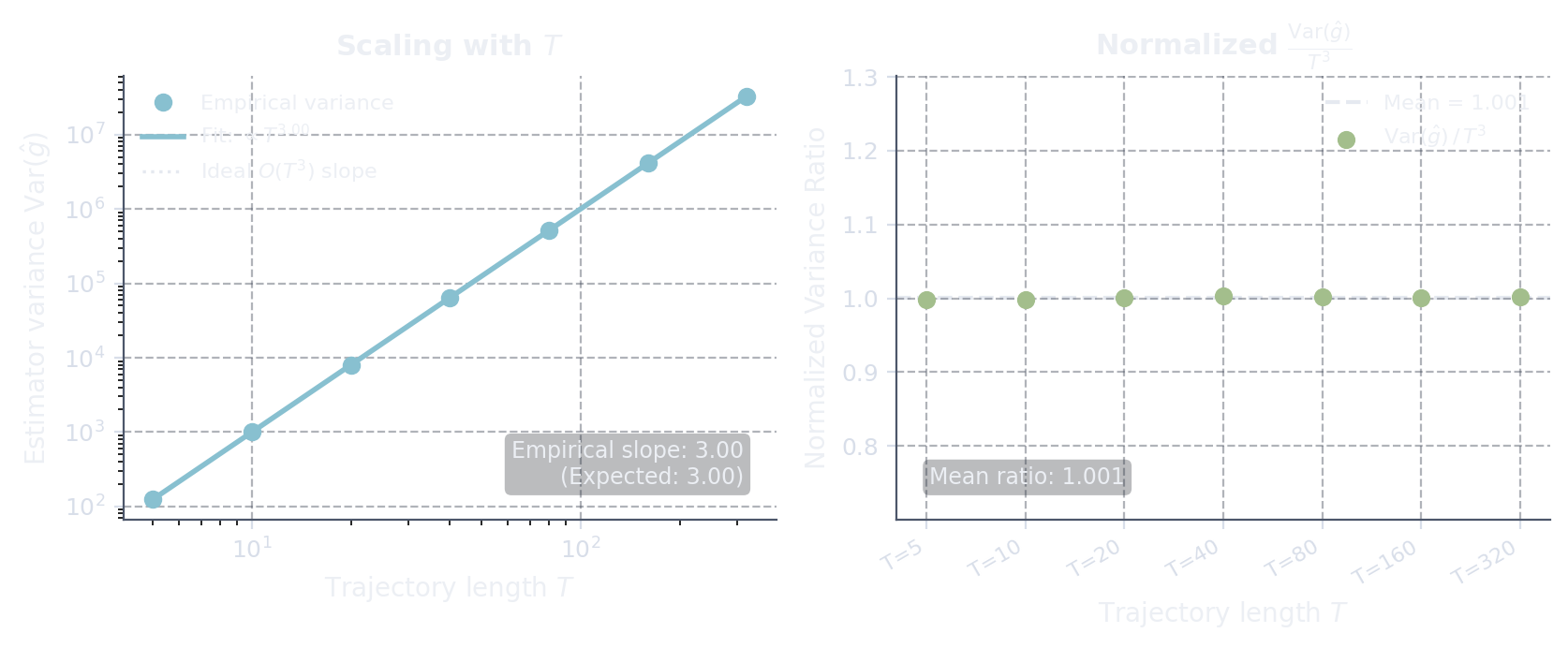
The setup is as follows: at each time step, the agent observes a state $s_t$ drawn uniformly from $[-1, 1]^4$ and selects one of $|\mathcal{A}| = 4$ actions according to a softmax linear policy $\pi_\theta(a | s) \propto \exp(\theta_a^\top s)$, with parameters $\theta$ drawn from a normal distribution $\mathcal{N}(0, 0.01^2)$. Each step yields a reward $r(s_t, a_t) = 1 + 0.1 \, \theta_{a_t}^\top s_t$. For each trajectory length $T \in \{5, 10, 20, 40, 80, 160, 320\}$, we estimate $\text{Var}(\hat{g})$ from 30,000 independent trajectories:

• Left: Log-log plot of gradient estimator variance $\text{Var}(\hat{g})$ versus trajectory length $T$, yielding an empirical scaling exponent of $3.00$.
• Right: Normalized variance $\frac{\text{Var}(\hat{g})}{T^3}$ across various values of $T$, confirming that the ratio remains tightly around a constant.

"""
Generate a 2-panel figure illustrating REINFORCE variance scaling with trajectory length T: Var(g) = O(T^3).

Setup: Multi-step environment with softmax linear policy.
  - State features: s_t ~ Uniform([-1, 1]^n), with fixed n = 4.
  - Policy: softmax linear pi_theta(a | s) = exp(theta_a^T s) / sum_a' exp(theta_{a'}^T s)
  - Number of actions: |A| = 4 (fixed)
  - theta initialized near zero
  - Reward per step: r(s_t, a_t) = 1 + 0.1 * (theta_{a_t}^T s_t)  (mean reward ~ 1)
  - Score: X_t = (e_{a_t} - pi_t) ⊗ s_t
  - Estimator: g(tau) = R(tau) * S(tau) where S = sum_t X_t
"""

import numpy as np
import matplotlib
matplotlib.use("Agg")
import matplotlib.pyplot as plt
from scipy.special import softmax

# Color palette (Dark theme / Nord palette)
BG_COLOR_FIG = "#1E222A"    # Outer figure background
BG_COLOR_AX = "#252931"     # Subplot panel background
COLOR_TEXT = "#ECEFF4"      # Primary text color
COLOR_MUTED = "#D8DEE9"     # Muted text color
GRID_COLOR = "#3B4252"      # Grid line color
SPINE_COLOR = "#4C566A"     # Border / spine color

COLOR_T = "#88C0D0"         # Nord cyan/blue
COLOR_RATIO = "#A3BE8C"     # Nord green
COLOR_REF = "#E5E9F0"       # Dotted reference line


def simulate_reinforce_gradients(n_samples, T, n_feat, n_actions, rng):
    """
    Simulates trajectories and returns the REINFORCE gradient estimates.
    The policy theta is kept identical using a fixed seed generator.
    """
    theta_rng = np.random.default_rng(0)
    theta = theta_rng.normal(0, 0.01, (n_actions, n_feat))
    d = n_actions * n_feat

    total_scores = np.zeros((n_samples, d))
    total_rewards = np.zeros(n_samples)

    for t in range(T):
        # Sample states: (n_samples, n_feat)
        states = rng.uniform(-1, 1, (n_samples, n_feat))

        # Compute logits and action probabilities: (n_samples, n_actions)
        logits = states @ theta.T
        probs = softmax(logits, axis=1)

        # Sample actions using cumulative probability thresholding
        cum_probs = np.cumsum(probs, axis=1)
        u = rng.uniform(0, 1, n_samples)
        actions = np.sum(cum_probs < u[:, None], axis=1)
        actions = np.clip(actions, 0, n_actions - 1)

        # Compute scores: (e_{a_t} - pi_t) ⊗ s_t
        e_a = np.zeros((n_samples, n_actions))
        e_a[np.arange(n_samples), actions] = 1.0
        diff = e_a - probs

        # Kronecker product: each row of diff ⊗ each row of states
        score_vecs = diff[:, :, None] * states[:, None, :]
        score_vecs = score_vecs.reshape(n_samples, d)
        total_scores += score_vecs

        # Compute step rewards: 1.0 + 0.1 * (theta_a^T s_t)
        theta_a = theta[actions]
        rewards = 1.0 + 0.1 * np.sum(theta_a * states, axis=1)
        total_rewards += rewards

    # REINFORCE estimator: g = R(tau) * S(tau)
    return total_rewards[:, None] * total_scores


def reinforce_variance(n_samples, T, n_feat, n_actions, seed=42):
    """
    Computes the variance of the REINFORCE gradient estimator for trajectory length T.
    """
    rng = np.random.default_rng(seed)
    all_g = simulate_reinforce_gradients(n_samples, T, n_feat, n_actions, rng)
    return np.var(all_g, axis=0).sum()


def run_variance_experiment(T_list, n_samples, n_feat, n_actions):
    """
    Runs the simulation over multiple trajectory lengths T.
    """
    var_vs_T = []
    for T in T_list:
        print(f"Running simulation for T={T}...")
        var_g = reinforce_variance(n_samples, T, n_feat, n_actions, seed=42)
        var_vs_T.append(var_g)
    return np.array(var_vs_T)


def plot_variance_scaling(T_list, var_vs_T, output_path):
    """
    Plots the variance scaling results in a 2-panel figure.
    """
    log_T = np.log(T_list)
    log_var_T = np.log(var_vs_T)
    slope_T, intercept_T = np.polyfit(log_T, log_var_T, 1)
    print(f"\nEmpirical slope wrt T: {slope_T:.4f}")

    ratios = var_vs_T / (T_list ** 3)
    mean_ratio = np.mean(ratios)
    print(f"Mean normalized ratio Var(g)/T^3: {mean_ratio:.4f}")

    fig, (ax1, ax2) = plt.subplots(1, 2, figsize=(8.5, 3.6))

    for ax in (ax1, ax2):
        ax.set_facecolor("none")
        ax.spines["top"].set_visible(False)
        ax.spines["right"].set_visible(False)
        ax.spines["left"].set_color(SPINE_COLOR)
        ax.spines["bottom"].set_color(SPINE_COLOR)
        ax.tick_params(colors=COLOR_MUTED, labelsize=9)
        ax.grid(True, linestyle="--", alpha=0.4, color=GRID_COLOR)

    fig.patch.set_facecolor("none")

    # --- Panel 1: Var vs T ---
    ax1.loglog(T_list, var_vs_T, "o", color=COLOR_T, ms=6, label="Empirical variance", zorder=3)
    fit_T = np.exp(intercept_T) * (T_list ** slope_T)
    ax1.loglog(T_list, fit_T, "-", color=COLOR_T, lw=2, label=f"Fit: $\\propto T^{{{slope_T:.2f}}}$", zorder=2)
    # Reference line T^3
    ref_T = var_vs_T[0] * (T_list / T_list[0])**3
    ax1.loglog(T_list, ref_T, ":", color=COLOR_REF, lw=1.2, label=r"Ideal $O(T^3)$ slope", zorder=1)

    ax1.set_xlabel("Trajectory length $T$", fontsize=10, color=COLOR_TEXT)
    ax1.set_ylabel(r"Estimator variance $\mathrm{Var}(\hat{g})$", fontsize=10, color=COLOR_TEXT)
    ax1.set_title(r"Scaling with $T$", fontsize=11, fontweight="bold", color=COLOR_TEXT, pad=8)
    leg1 = ax1.legend(fontsize=8, loc="upper left", frameon=False)
    plt.setp(leg1.get_texts(), color=COLOR_TEXT)

    ax1.text(0.95, 0.08, f"Empirical slope: {slope_T:.2f}\n(Expected: 3.00)",
             transform=ax1.transAxes, fontsize=8.5, color=COLOR_TEXT, ha="right",
             bbox=dict(boxstyle="round,pad=0.3", facecolor="#1E222A", alpha=0.3, edgecolor="none"))

    # --- Panel 2: Normalized ratio Var(g) / T^3 ---
    x_pos = np.arange(len(T_list))
    ax2.axhline(mean_ratio, color=COLOR_REF, lw=1.5, ls="--", label=f"Mean = {mean_ratio:.3f}", zorder=1)
    ax2.scatter(x_pos, ratios, color=COLOR_RATIO, s=35, zorder=3, label=r"$\mathrm{Var}(\hat{g})\,/\,T^3$")
    ax2.set_xticks(x_pos)
    ax2.set_xticklabels([f"T={t}" for t in T_list], rotation=30, ha="right", fontsize=8)
    ax2.set_ylim(mean_ratio * 0.7, mean_ratio * 1.3)
    ax2.set_xlabel("Trajectory length $T$", fontsize=10, color=COLOR_TEXT)
    ax2.set_ylabel(r"Normalized Variance Ratio", fontsize=10, color=COLOR_TEXT)
    ax2.set_title(r"Normalized $\frac{\mathrm{Var}(\hat{g})}{T^3}$", fontsize=11, fontweight="bold", color=COLOR_TEXT, pad=8)
    leg2 = ax2.legend(fontsize=8, loc="upper right", frameon=False)
    plt.setp(leg2.get_texts(), color=COLOR_TEXT)

    ax2.text(0.05, 0.08, f"Mean ratio: {mean_ratio:.3f}",
             transform=ax2.transAxes, fontsize=8.5, color=COLOR_TEXT, ha="left",
             bbox=dict(boxstyle="round,pad=0.3", facecolor="#1E222A", alpha=0.3, edgecolor="none"))

    plt.tight_layout()
    plt.savefig(output_img_path, dpi=200, bbox_inches="tight", transparent=True)
    print(f"\nSaved 2-panel figure to {output_img_path}")


if __name__ == "__main__":
    n_samples = 30000
    n_actions = 4
    n_feat = 4
    T_list = np.array([5, 10, 20, 40, 80, 160, 320])
    output_img_path = "/Users/pedregosa/dev/webpage/content/images/2026/reinforce_variance_scaling.png"

    var_vs_T = run_variance_experiment(T_list, n_samples, n_feat, n_actions)
    plot_variance_scaling(T_list, var_vs_T, output_img_path)
        

The message here is that the $\mathcal{O}(T^3)$ upper bound doesn't seem to be wildly pessimistic, but painfully accurate. Fitting a power law on a log-log scale matches the theoretical $O(T^3)$ bound with remarkable precision.

Summary

The central achievement of the REINFORCE algorithm is that it allows us to optimize policies without knowing or differentiating through the environment's transition dynamics. By applying the log-derivative trick, the product of transition probabilities turns into a sum, and all environment-dependent terms drop out.

However, the price we pay for this model-free elegance is high variance. Specifically, as we derived above, the variance of the REINFORCE estimator scales cubically with the trajectory length ($O(T^3)$). This stems from the combination of a return $R(\tau)$ that grows linearly with $T$ (contributing an $O(T^2)$ term when squared) and a sum of score vectors $S(\tau)$ whose variance also grows linearly as $O(T)$ due to uncorrelated steps. As a result, even a moderate increase in the episode horizon $T$ leads to a massive explosion in variance, requiring a prohibitively large number of samples to obtain stable gradient estimates.

In the next post we'll cover some techniques to reduce the variance of this estimator.

References