On the Convergence of the Unadjusted Langevin Algorithm
Insights From the Quadratic Model
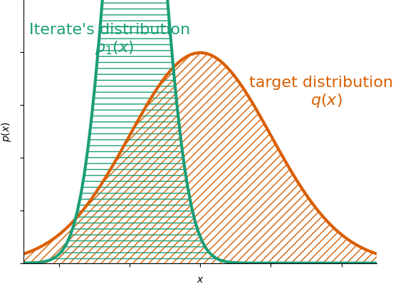
The Langevin algorithm is a simple and powerful method to sample from a probability distribution. It's a key ingredient of some machine learning methods such as diffusion models and differentially private learning. In this post, I'll derive a simple convergence analysis of this method in the special case when the target distribution is a Gaussian distribution. This analysis will reveal some surprising properties of this algorithm. For example, we'll show that the iterates don't converge to the target distribution, but instead converge to a distribution whose distance to the target distribution is proportional to the step-size.
The Unadjusted Langevin Algorithm (ULA)
The Langevin algorithm –also known as Langevin Monte Carlo and Langevin MCMC– is an algorithm for generating samples from a
probability distribution for which we have access to the gradient of its log probability. It's behind some of the recent success of generative AI such as diffusion models
Given a function $f: \RR^d \to \RR$ for which we have access to its gradient $\nabla f$, and where $\int \exp(-f(x)) \dif x$ is finite, the Langevin algorithm produces a sequence of random iterates $x_0, x_1, \ldots$ with associated density function $x_0 \sim p_0, x_1 \sim p_1, \ldots$ increasingly approximates the following target distribution: \begin{equation*} q(x) \defas \frac{1}{Z} \exp \left( -\mathcal{f}(x) \right)\,, \quad \text{ with } Z \defas \int_{\RR^p} \exp(-f(x)) \dif x\,. \end{equation*}
And it does so in a remarkable simple way:
Unadjusted Langevin Algorithm (ULA)
Input: starting guess $x_0 \in \RR^d$ and step-size $\step \gt 0$.
For $t=0, 1, \ldots$
\begin{equation}\label{eq:ula}
\begin{aligned}
& \text{sample } {\color{colorepsdp}\boldsymbol{\varepsilon}_t} \sim \mathcal{N}(0, I)\\
&x_{t+1} = x_t - \step \nabla f(x_t) + \sqrt{2 \step} {\color{colorepsdp}\boldsymbol{\varepsilon}_t}
\end{aligned}
\end{equation}
The algorithm is sometimes also referred to as noisy gradient descent, because it's just that: gradient descent with some Gaussian noise added to the gradient at each iteration.
Although we won't use this perspective in this blog post, it also corresponds to the Euler-Maruyama discretization of a Langevin diffusion process (hence the name).
Paul Langevin (1872 - 1946) was a French physicist who developed Langevin dynamics and the Langevin equation. He was a doctoral student of Pierre Curie and later a lover of widowed Marie Curie. He is also known for his two US patents with Constantin Chilowsky in 1916 and 1917 involving ultrasonic submarine detection. He is entombed at the Panthéon.
The Langevin algorithm admits different variants, depending on whether the step-size is constant or decreasing and
whether there's a rejection step or not.
The variant above with a constant step-size $\step$ and no rejection step is the most commonly used in practice and is often referred to as the unadjusted Langevin algorithm (ULA). Although I won't cover them in this post, it's worth noting that there are also stochastic variants of the algorithm, where $\nabla f(x_t)$ is replaced with a stochastic unbiased estimator.
The goal of this post is to characterize the speed of convergence of the iterates towards this target distribution. We'll identify the key properties that influence this convergence, and see a few surprises along the way.
The Difficulty of Analyzing the Langevin Algorithm
One of the key differences between the analysis of optimization and that of sampling algorithms is that in sampling
algorithms, we're not looking to bound the distance between the iterates and the optimal solution. Instead, we're
looking to bound the distance between the iterates' distribution and the target distribution. This has far-reaching consequences. For once, distances between distributions are
often difficult to compute. As an example, the squared Wasserstein (also known as Kantorovich-Rubinstein) $W_2(, )^2$ distance between probability distributions
$\probaone$ and $\probatwo$ is defined as
\begin{equation}
W_2(\probaone, \probatwo)^2 \defas \inf_{\pi \in \Pi(\probaone, \probatwo)} \EE_{(x,
y) \sim \pi} {\|x - y\|}^2\,,
\end{equation}
where $\Pi(\probaone, \probatwo)$ is the set of all couplings between $\probaone$ and $\probatwo$.
Fortunately, computing the Wasserstein distance of Gaussian distributions admits an explicit formula. When
$\probaone$ and $\probatwo$ are both Gaussian with mean $\mu_p$,
$\mu_q$ and covariance $\Sigma_p$,
$\Sigma_q$ respectively, the Wasserstein distance between them can be expressed as
by
It's Gaussians all the Way

Throughout the rest of the post we'll assume that $f$ is a quadratic function of the form: \begin{equation}\label{eq:quadratic_function} f(x) \defas \frac{1}{2}(x - {\mu}_q) H (x - {\mu}_q)\,. \end{equation} with a positive definite matrix $H$. The associated target distribution $q(x) \propto \exp \left( -\mathcal{f}(x) \right)$ is then a Gaussian distribution with mean ${\mu}_q$ and covariance $H^{-1}$.
Similar to the analysis of optimization methods on quadratics, the analysis of ULA simplifies considerably when the target measure is Gaussian, as in this case each step of the algorithm is equivalent to a Gaussian random walk. Assuming that $x_0$ is sampled from a Gaussian distribution, the first iterate is then a linear combination of two Gaussian random variable, which is again a Gaussian random variable. For the same reason, any future iterate is also a Gaussian random variable.
Unroll all the things!
One advantage of working with Gaussian target measures is that we can write down any iterate in a simple non-recursive formula. In this case the gradient $\nabla f(x) = H (x - \mu_q)$ is an affine function of the parameters, which allows us to unroll
the iterates as
\begin{align}
x_{t} - \mu_q &= (I - \step H) (x_{t-1} - \mu_q) + \sqrt{2 \step}
{\color{colorepsdp}\boldsymbol{\varepsilon}_{t-1}}\\
&= (I - \step H) \left( (I - \step H) (x_{t-2} - \mu_q) + \sqrt{2 \step}
{\color{colorepsdp}\boldsymbol{\varepsilon}_{t-2}}\right) + \sqrt{2 \step}
{\color{colorepsdp}\boldsymbol{\varepsilon}_{t-1}}\\
&= (I - \step H)^2 (x_{t-2} - \mu_q) + \sqrt{2 \step} (I - \step
H){\color{colorepsdp}\boldsymbol{\varepsilon}_{t-2}} + \sqrt{2 \step}
{\color{colorepsdp}\boldsymbol{\varepsilon}_{t-1}} \\
&= \cdots\\
&= (I - \step H)^t (x_0 - \mu_q) + \sqrt{ 2 \step} \sum_{i=0}^{t-1} (I - \step H)^{t - 1 - i}
{\color{colorepsdp}\boldsymbol{\varepsilon}_{i}}\,, \label{eq:last_eq_unrolling}
\end{align}
where in the first line we've used the definition of $x_t$, in the second one that of $x_{t-1}$ and so on.
We now want to characterize the distribution of the iterates. Thanks to the previous section, we know that this is a
Gaussian distribution, so it is fully determined through its mean $\mu_t$ and covariance
$\Sigma_t$. Let's estimate these two quantities separately. For simplicity, we'll assume that the initial iterate was sampled from a Gaussian distribution with scaled identity covariance, that is, $p_0 = \mathcal{N}(\mu_0, \sigma^2 I)$ for some scalar $\sigma \geq 0$.
1️⃣: mean. Taking expectations on \eqref{eq:last_eq_unrolling}, all the terms in ${\color{colorepsdp}\boldsymbol{\varepsilon}_{i}}$ vanish, and we are left with \begin{equation}\label{eq:mean_t} \mu_t - \mu_q \stackrel{\eqref{eq:last_eq_unrolling}}{=} (I - \step H)^t (\mu_0 - \mu_q)\,, \end{equation} As long as the spectral radius of $I - \step H$ is smaller than $1$, the right hand side vanishes exponentially fast. Hence the formula above tells us that the iterate average $\mu_t$ converges exponentially fast to the target mean $\mu_q$.
2️⃣: covariance. This one's more difficult. Using the shorthand notation $x^2 = x x^\top$ for a vector $x$, we have \begin{align} \Sigma_t &\defas \EE (x_t - \mu_t)^2 = \EE\biggl((I - \step H)^t (x_0 - \mu_q) + \sqrt{ 2 \step} \sum_{i=0}^{t-1} (I - \step H)^{t-1-i} {\color{colorepsdp}\boldsymbol{\varepsilon}_{i}} - (\mu_t - \mu_q)\biggl)^2 \\ &\stackrel{\eqref{eq:mean_t}}{=} \EE\left((I - \step H)^t (x_0 - \mu_0) + \sqrt{ 2 \step} \sum_{i=0}^{t-1} (I - \step H)^{t-1-i} {\color{colorepsdp}\boldsymbol{\varepsilon}_{i}} \right)^2 \\ &= 2 \step \sum_{i=0}^{t-1} (I - \step H)^{2i} + \sigma^2 (I - \step H)^{2t}\\ &= \underbrace{( H - \frac{\step}{2} H^2)^{-1}}_{\text{biased covariance}} + \underbrace{(I - \step H)^{2t} [\sigma^2 I - ( H - \frac{\step}{2} H^2)^{-1}]}_{\text{vanishing as $t \to \infty$}} \,, \label{eq:limit_covariance} \end{align} where in the third line we've used the fact that the $\boldsymbol{\varepsilon}_i$ are independent, and so the terms $\EE[{\color{colorepsdp}\boldsymbol{\varepsilon}_{i}} {\color{colorepsdp}\boldsymbol{\varepsilon}_{j}}^\top]$ vanish for $i \neq j$. In the last line we've used the formula for the partial sum of a geometric series $\sum_{i=0}^{t-1} A^i = (I - A)^{-1} - A^t (I - A)^{-1}$, with $A = (I - \step H)^2$.
As $t \to \infty$, the second term vanishes and only the first one survives. Interestingly, this last term is not the covariance matrix of the stationary distribution $H^{-1}$, as one would expect from a converging algorithm. Instead, the iterates' covariance converges towards $( H - \frac{\step}{2} H^2)^{-1}$, which only equals the stationary $H^{-1}$ in the limit as $\step \to 0$. Because of this mismatch, we say that ULA is a biased algorithm.
Convergence Rate to the Biased Limit
In the last section we've seen that the iterates of ULA converge to a Gaussian distribution with mean $\mu_q$ and covariance $( H - \frac{\step}{2} H^2)^{-1}$. We'll now quantify the speed of this convergence.
As is customary for optimization results, this convergence rate will depend on the extremal eigenvalues of the Hessian's loss (which in this case is also the target distribution's precision matrix). Let $\ell$ and $L$ denote a lower and upper bound on $H$'s eigenvalues respectively. With this, we have the following result.
Let $p_t$ denote the distribution of the iterates of ULA with step-size $\step$ on a quadratic objective function, where the initial guess $p_0$ is a Gaussian distribution with covariance $\sigma^2 I$, $\sigma \leq L(1 + \frac{\step}{2}L)$.
Then, ULA converges exponentially fast in the Wasserstein distance towards $p_{\step}$, a Gaussian distribution with mean $\mu_q$ and covariance $( H - \frac{\step}{2} H^2)^{-1}$. More precisely, for any $\step \lt 2/L$ we have
\begin{align}
W_2(p_t, p_{\step}) &\leq \left(\max\{|1 - \step L|, |1 - \step \ell|\}\right)^{t} W_2(p_0, p_{\step})\,. \label{eq:convergence_rate}
\end{align}
From the formula for the Wasserstein distance between Gaussian distributions \eqref{eq:wasserstein_simple}, the total distance decomposes into the sum of the distance of the means and that of its square root covariance. We'll estimate these two terms separately.
1️⃣: distance between means. For this distance we have \begin{align} \|\mu_t - \mu_q\|^2 &\stackrel{\eqref{eq:mean_t}}{=} \|(I - \step H)^t (\mu_0 - \mu_q) \|^2 \\ &\leq \max\{|1 - \step L|, |1 - \step \ell|\}^{2t} \|\mu_0 - \mu_q\|^2 \\ \end{align} where the last line follows by Cauchy-Schwartz.
2️⃣: distance between covariances. Let $Q \diag(h_1, \ldots, h_d) Q^\top$ be the eigendecomposition of $H$, where $h_1, h_2, \ldots$ are the eigenvalues of $H$ and $Q$ is an orthonormal matrix. We'll first show that both $(H - \frac{\step}{2} H^2)^{-1}$ and $\Sigma_t$ are diagonal in the same basis as this will simplify the computation of the Frobenius norm of their difference.
Replacing $H$ by its eigendecomposition in the formula of the biased covariance, we have that this last one admits the following eigendecomposition: \begin{align} (H - \frac{\step}{2} H^2)^{-1} &= Q \diag(\frac{1}{h^\step_1}, \ldots, \frac{1}{h^\step_d}) Q^\top \,, \end{align} with $h_i^\step \defas h_i - \frac{\step}{2}h_i^2$. Also replacing $H$ by its eigendecomposition in \eqref{eq:limit_covariance}, we obtain that $\Sigma_t$ admits the eigendecomposition \begin{align} \Sigma_t = Q \bigl(\diag(\frac{1}{h^\step_1} - z_1, \ldots, \frac{1}{h^\step_d} - z_d)\bigl)Q^\top \,, \end{align} with $z_i \defas (1 - \step h_i)^{2 t}(\frac{1}{h_i^\step} - \sigma^2)$.
Now using the fact that the squared Frobenius norm of a matrix is the sum of its eigenvalues, we can write the distance between the two covariances in terms of $h_i^\step$ and $z_i$: \begin{align} &\|\Sigma_t^{1/2} - ( H - \frac{\step}{2} H^2)^{-1/2}\|_F^2 \nonumber\\ &\quad= \sum_{i=1}^d \biggl(\sqrt{\frac{1}{h^\step_i} - z_i} - \sqrt{\frac{1}{h^{\step}_i}}\biggl)^2 \\ &\quad= \sum_{i=1}^d \frac{1}{h^\step_i}\biggl(2 - h_i^\step z_i - 2 \sqrt{1 - h_i^\step z_i} \biggl) \label{eq:expanding_square}\\ &\quad\leq \sum_{i=1}^d \frac{1}{h^\step_i}\biggl(2 - h_i^\step z_i - 2 (1 - h_i^\step z_i) \biggl) \label{eq:sqrt_inequality}\\ &\quad= \sum_{i=1}^d z_i = \sum_{i=1}^d (1 - \step h_i)^{2 t}(\frac{1}{h^\step_i} - \sigma^2)\\ &\quad\leq \max\{|1 - \step L|, |1 - \step \ell|\}^{2t} \underbrace{\sum_{i=1}^d (\frac{1}{h^\step_i} - \sigma^2)}_{= \|(H - \frac{\step}{2} H^2)^{-1} - \sigma^2 I\|_F^2}\,, \end{align} where in \eqref{eq:expanding_square} we have expanded the square and in \eqref{eq:sqrt_inequality} we have used the inequality $\sqrt{1 - x} \geq 1 - x$ for $x \in [0, 1]$, together with the assumption $\sigma^2 \leq h^\step_i$.
Finally, we sum the bound in the distance between means and the bound in the distance between covariances to obtain \begin{equation} W_2(p_0, p_{\step})^2 \leq \max\{|1 - \step L|, |1 - \step \ell|\}^{2t} \underbrace{\bigl(\|\mu_0 - \mu_q\|^2 + \|(H - \frac{\step}{2} H^2)^{-1} - \sigma^2 I\|_F^2\bigl)}_{=W_2(p_0, p_{\step})^2}\,. \end{equation} The final result then comes from taking the square root on both sides.
Convergence Rate to the Stationary Distribution
The rate in the last lemma unfortunately only bounds the distance to the biased limit. However, usually we'll instead want the distance to the target distribution since that's the distribution we want to sample from. The Wasserstein distance (as any distance) satisfies the triangular inequality. We can then use this inequality to bound on the distance to the target distribution: \begin{equation} W_2(p_t, q) \leq W_2(p_t, p_{\step}) + W_2(p_{\step}, q)\,. \end{equation} Of the two terms in the right hand side, the first one is already bounded by the previous lemma. The second one is the distance between the biased limit and the target distribution. By bounding this last term we can achieve our goal, which was to bound the distnace between $p_t$ and the target distribution. As in the previous Lemma, we denote by $\ell$ and $L$ a lower and upper bound on $H$'s eigenvalues respectively.
Let $p_t$ denote the distribution of the iterates of ULA with step-size $\step$ on a quadratic objective function, where the initial guess $p_0$ is a Gaussian distribution with covariance $\sigma^2 I$, $\sigma \leq L(1 + \frac{\step}{2}L)$.
Then, for any step-size $\step \lt 2/L$, the Wasserstein distance between $p_t$ and the target distribution $q$ can be bounded by a sum of two terms, of which the first one vanishes exponentially fast in $t$, while the second one is $\mathcal{O}(\step)$ close to the target distribution. More precisely, at every iteration $t$ we have
\begin{equation}
W_2(\probaone_t, \probatwo) \leq \underbrace{\rho^{t}\, W_2(p_0, p_{\step})\vphantom{\frac{1}{2}}}_{\text{exponential convergence}} + \underbrace{\frac{\step}{4}\sqrt{\tr(H)}}_{\text{stationary}} \,,
\end{equation}
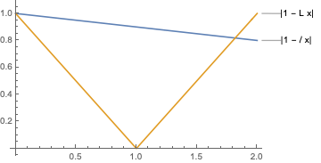
with linear rate factor $\rho \defas \max\{|1 - \step L|,|1 - \step \ell|\}$.
As in the proof of the previous lemma, we denote the eigenvalues of $H$ by $h_1, h_2, \ldots$.
We'll now bound the distance between $p_{\step}$ and the target distribution $q$. Both distributions are Gaussians with mean $\mu_q$, so their Wasserstein distance is the Frobenius norm of the difference of their square root covariances \eqref{eq:wasserstein_simple}. Then we have:
\begin{align}
W_2(q, p_{\step})^2 &= \|H^{-1/2} - ( H - \frac{\step}{2} H^2)^{-1/2}\|_F^2 \\
&= \sum_{i=1}^d \frac{1}{h_i}\biggl(1-\frac{1}{\sqrt{1 + \frac{1}{2} \step h_{i}}}\biggl)^2\,.\label{eq:wasserstein_bias_eigvals}
\end{align}
Let's now consider the function $\varphi(z) = (1 - \frac{1}{\sqrt{1 + z}})^2$ for $z$ in the $[0, 1]$ interval.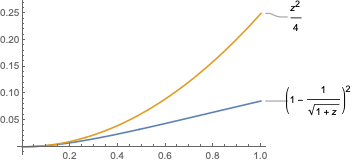
We can now use this bound on $\varphi$ to upper bound the terms inside the parenthesis of \eqref{eq:wasserstein_bias_eigvals} as follows: \begin{align} W_2(q, p_{\step})^2 &\stackrel{\eqref{eq:wasserstein_bias_eigvals}}{=} \sum_{i=1}^d \frac{1}{h_i}\biggl(1-\frac{1}{\sqrt{1 + \frac{1}{2} \step h_{i}}}\biggl)^2 \\ &\stackrel{\eqref{eq:bound_varphi}}{\leq} \frac{\step^2}{16} \underbrace{\sum_{i=1}^d h_i}_{= \tr(H)} \end{align}
Finally, taking the square root of the bound above and combining it with the previous lemma we get the desired result.
The result above shows how the convergence rate of Langevin can be split into a sum of two terms, the first one being an exponentially fast convergence and the other is stationary. Although this fact is widely known, the result above seems to be somewhat new in that it doesn't have have higher order terms in $\step$ as (Wibisono 2018).
The formula above establishes convergence for any step-size $\gamma \lt 2/L$. However, for most except the very large step-sizes it can be further simplified. For example, for $\step \leq 2 / (L + \ell)$ we have that $|1 - \step \ell| \geq |1 - \step L|$. In this case, the $\max$ in the Theorem can simplifies to $ \max\{|1 - \step L|,|1 - \step \ell|\} = 1 - \step \ell$
Under the same assumptions of the theorem above, for any step-size $\step \leq 2 / (L + \ell)$ we have \begin{equation} W_2(\probaone_t, \probatwo) \leq \vphantom{\frac{1}{2}}(1 - \step \ell)^{t} W_2(p_0, p_{\step}) + \frac{\step}{4}\sqrt{\tr(H)} \,. \end{equation}
The formula above shows how the convergence of the Langevin algorithm can be split onto the sum of two terms, one of which is exponentially decreasing, and the other one is a non-zero bias term. In particular this shows that ULA is a biased algorithm, even in the case of Gaussian target distributions.
The bias term is proportional to the step-size. In particular, the bias vanishes when the step-size is zero but is positive otherwise. This is one defining difference between gradient descent and the ULA algorithm: in gradient descent, a non-zero step-size still takes you to the right minimizer, while ULA will be biased. If one wishes to eliminate the bias, one could use a decreasing step-size or to change the algorithm to include a rejection step –the so-called Metropolis-adjusted Langevin algorithm (MALA).
To know more
The literature on the analysis of ULA is vast, so I won't cover it all but merely point to some of my favorite papers. For any notable omission, please leave a comment below!
Early works that derive convergence rates for ULA on convex and smooth functions (that is, more general than the quadratic setting of this post) include those of Durmus et al.
A very insightful work that already derived an asymptotic $\frac{\step}{4}\sqrt{\tr(H)} + \mathcal{O}(\step^2)$ bias of Langevin on quadratics is that of Wibisono.
Another aspect worth mentioning is that most analyses of ULA bound the bias in terms of the problem dimensionality,
Citing
If you find this blog post useful, please consider citing as
On the Convergence of the Unadjusted Langevin Algorithm, Fabian Pedregosa, 2023
with bibtex entry:
    @misc{pedregosa2023ulaq,
      title={On the Convergence of the Unadjusted Langevin Algorithm},
      author={Fabian Pedregosa},
      howpublished = {\url{http://fa.bianp.net/blog/2023/ulaq/}},
      year={2023}
    }
Acknowledgements
Thanks to Baptiste Goujaud for reporting numerous typos and to Courtney Paquette, James Harrison and Sam Power for feedback on the blog post.