Ridge regression path
Ridge coefficients for multiple values of the regularization parameter can be elegantly computed by updating the thin SVD decomposition of the design matrix:
import numpy as np
from scipy import linalg
def ridge(A, b, alphas):
    """
    Return coefficients for regularized least squares

         min ||A x - b||^2 + alpha ||x||^2

    Parameters
    ----------
    A : array, shape (n, p)
    b : array, shape (n,)
    alphas : array, shape (k,)

    Returns
    -------
    coef: array, shape (p, k)
    """
    U, s, Vt = linalg.svd(X, full_matrices=False)
    d = s / (s[:, np.newaxis].T ** 2 + alphas[:, np.newaxis])
    return np.dot(d * U.T.dot(y), Vt).T
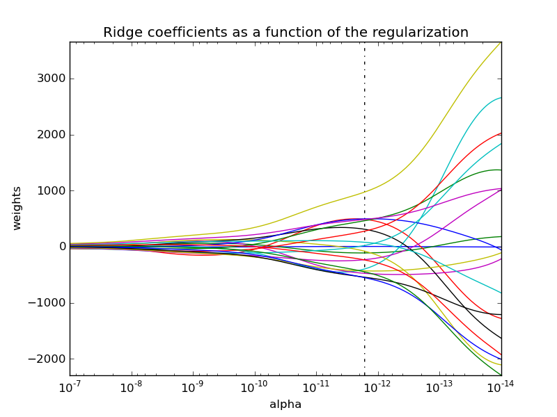
This can be used to efficiently compute what it's regularization path, that is, to plot the coefficients as a function of the regularization parameter. Since the bottleneck of the algorithm is the singular value decomposition, computing the coefficients for other values of the regularization parameter basically comes for free.

A variant of this algorithm can then be used to compute the optimal regularization parameter in the sense of leave-one-out cross-validation and is implemented in scikit-learn's RidgeCV (for which Mathieu Blondel has an excelent post by ). This optimal parameter is denoted with a vertical dotted line in the following picture, full code can be found here.