We can tighten the analysis of gradient descent with momentum through a cobination of Chebyshev polynomials of the first and second kind. Following this connection, we'll derive one of the most iconic methods in optimization: Polyak momentum.

Gradient Descent with Momentum

Gradient descent with momentum, also known as heavy ball or momentum for short, is an optimization method designed to solve unconstrained optimization problems of the form \begin{equation} \argmin_{\xx \in \RR^d} f(\xx)\,, \end{equation} where the objective function $f$ is differentiable and we have access to its gradient $\nabla f$. In this method the udpate is a sum of two terms. The first term is the difference between current and previous iterate $(\xx_{t} - \xx_{t-1})$, also known as momentum term. The second term is the gradient $\nabla f(\xx_t)$ of the objective function.

Gradient Descent with Momentum
Input: starting guess $\xx_0$, step-size ${\color{colorstepsize} h} > 0$ and momentum parameter ${\color{colormomentum} m} \in (0, 1)$.
$\xx_1 = \xx_0 - \dfrac{{\color{colorstepsize} h}}{1 + {\color{colormomentum} m}} \nabla f(\xx_0)$
For $t=1, 2, \ldots$ compute \begin{equation}\label{eq:momentum_update} \xx_{t+1} = \xx_t + {\color{colormomentum} m}(\xx_{t} - \xx_{t-1}) - {\color{colorstepsize} h}\nabla f(\xx_t) \end{equation}

Gradient descent with momentum has seen a renewed interest in recent years, as a stochastic variant that replaces the true gradient with a stochastic estimate has shown to be very effective for deep learning.

Quadratic model

Although momentum can be applied to any problem with a twice differentiable objective, in this post we'll assume for simplicity the objective function $f$ quadratic.The extension to non-quadratic functions follows simple local arguments and can be found for example in Polyak's book The quadratic assumption is restrictive, but well worth it, as it allows a richer theory and a simplified analysis through the connection between optimization methods and polynomials. As in the previous post, we'll assume the objective is \begin{equation}\label{eq:opt} f(\xx) \defas \frac{1}{2}\xx^\top \HH \xx + \bb^\top \xx~, \end{equation} where $\HH$ is a positive definite square matrix with eigenvalues in the interval $[\lmin, L]$.

Example: Polyak Momentum, also known as the HeavyBall method, is a widely used instance of momentum. Originally developed for the solution of linear equations and known as Frankel's method, it was generalized to general objectives and popularized in the optimization community by Boris Polyak.
Boris Polyak (1935 —) is a Russian mathematician and pioneer of optimization. Currently, he leads the Laboratory at Institute of Control Science in Moscow.

Polyak momentum follows the update \eqref{eq:momentum_update} with momentum and step-size parameters \begin{equation}\label{eq:polyak_parameters} {\color{colormomentum}m = {\Big(\frac{\sqrt{L}-\sqrt{\lmin}}{\sqrt{L}+\sqrt{\lmin}}\Big)^2}} \text{ and } {\color{colorstepsize}h = \Big(\frac{ 2}{\sqrt{L}+\sqrt{\lmin}}\Big)^2}\,, \end{equation} which gives the full algorithm

Polyak Momentum
Input: starting guess $\xx_0$, lower and upper eigenvalue bound $\lmin$ and $L$.
$\xx_1 = \xx_0 - {\color{colorstepsize}\frac{2}{L + \lmin}} \nabla f(\xx_0)$
For $t=1, 2, \ldots$ compute \begin{equation}\label{eq:polyak_momentum_update} \xx_{t+1} = \xx_t + {\color{colormomentum} {\Big(\tfrac{\sqrt{L}-\sqrt{\lmin}}{\sqrt{L}+\sqrt{\lmin}}\Big)^2}}(\xx_{t} - \xx_{t-1}) - {\color{colorstepsize} \Big(\tfrac{ 2}{\sqrt{L}+\sqrt{\lmin}}\Big)^2}\nabla f(\xx_t) \end{equation}

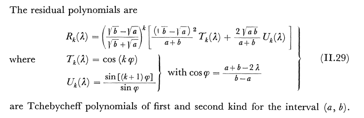
Residual Polynomials

In the last post we saw that to each gradient-based optimizer we can associate a sequence of polynomials $P_1, P_2, ...$ that we named residual polynomials and that determines the converge of the method:

Let $\xx_1, \xx_2, \ldots$ be the iterates generated by a momentum method and $P_1, P_2, \ldots$ the sequence of residual polynomials associated with this method. Then the error at each iteration $t$ verifies \begin{equation} \xx_t - \xx^\star = P_t(\HH)(\xx_0 - \xx^\star)\,. \end{equation}

This is a special case of the Residual polynomial Lemma proved in the last post.

In the last post we also gave an expression for this residual polynomial. Although this expression is rather involved in the general case, it simplifies for momentum, where it follows the simple recurrence:

Given a momentum method with parameters ${\color{colormomentum} m}$, ${\color{colorstepsize} h}$, the associated residual polynomials $P_0, P_1, \ldots$ verify the following recursion \begin{equation} \begin{split} &P_{t+1}(\lambda) = (1 + {\color{colormomentum}m} - {\color{colorstepsize} h} \lambda ) P_{t}(\lambda) - {\color{colormomentum}m} P_{t-1}(\lambda)\\ &P_0(\lambda) = 1\,,~ P_1(\lambda) = 1 - \frac{{\color{colorstepsize} h}}{1 + {\color{colormomentum}m}} \lambda \,. \end{split}\label{eq:def_residual_polynomial2} \end{equation}

A consequence of this result is that not only the method, but also its residual polynomial, has a simple recurrence. We will soon leverage this to simplify the analysis.

Chebyshev meets Chebyshev

Chebyshev polynomials of the first kind appeared in the last post when deriving the optimal worst-case method. These are polynomials $T_0, T_1, \ldots$ defined by the recurrence relation \begin{align} &T_0(\lambda) = 1 \qquad T_1(\lambda) = \lambda\\ &T_{k+1}(\lambda) = 2 \lambda T_k(\lambda) - T_{k-1}(\lambda)~. \end{align} A fact that we didn't use in the last post is that Chebyshev polynomials are orthogonal with respect to the weight function \begin{equation} \dif\omega(\lambda) = \begin{cases} \frac{1}{\pi\sqrt{1 - \lambda^2}} &\text{ if $\lambda \in [-1, 1]$} \\ 0 &\text{ otherwise}\,. \end{cases} \end{equation} That is, they verify the orthogonality condition \begin{equation} \int T_i(\lambda) T_j(\lambda) \dif\omega(\lambda) \begin{cases} > 0 \text{ if $i = j$}\\ = 0 \text{ otherwise}\,.\end{cases} \end{equation}

I mentioned that these are the Chebyshev polynomials of the first kind because there are also Chebyshev polynomials of the second kind, and although less used, also of the third kind, fourth kind and so on.

Chebyshev polynomials of the second kind, denoted $U_1, U_2, \ldots$, are defined by the integral \begin{equation} U_t(\lambda) = \int \frac{T_{t+1}(\xi) - T_{t+1}(\lambda)}{\xi- \lambda}\dif\omega(\xi)\,. \end{equation}

Although we will only use this construction for Chebyshev polynomials, it extends beyond this setup and is very natural because these polynomials are the numerators for the convergents of certain continued fractions.

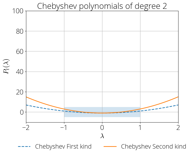
The polynomials of the second kind verify the same recurrence formula as the original sequence, but with different initial conditions. In particular, the Chebyshev polynomials of the second kind are determined by the recurrence \begin{align} &U_0(\lambda) = 1 \qquad U_1(\lambda) = 2 \lambda\\ &U_{k+1}(\lambda) = 2 \lambda U_k(\lambda) - U_{k-1}(\lambda)~. \end{align} Note how $U_1(\lambda)$ is different from $T_1$, but other than that, the coefficients in the recurrence are the same. Because of this, both sequences behave somewhat similarly, but also have important differences. For example, both kinds have extrema at the endpoints, but the value is different. For the first kind, the extrema is $\pm 1$, while for the second kind its $\pm (t+1)$.

Image of the first 6 Chebyshev polynomials of the first and second kind in the $[-1, 1]$ interval.

Momentum's residual polynomial

Time has finally come for the main result: the residual polynomial of gradient descent with momentum is nothing else than a combination of Chebyshev polynomials of the first and second kind. Since the properties of Chebyshev polynomials are well known, this will provide a way to derive convergence bounds for momentum.

Consider the momentum method with step-size ${\color{colorstepsize}h}$ and momentum parameter ${\color{colormomentum}m}$. The residual polynomial $P_t$ associated with this method can be written in terms of Chebyshev polynomials as \begin{equation}\label{eq:theorem} P_t(\lambda) = {\color{colormomentum}m}^{t/2} \left( {\small\frac{2 {\color{colormomentum}m}}{1 + {\color{colormomentum}m}}}\, T_t(\sigma(\lambda)) + {\small\frac{1 - {\color{colormomentum}m}}{1 + {\color{colormomentum}m}}}\, U_t(\sigma(\lambda))\right)\,, \end{equation} with $\sigma(\lambda) = {\small\dfrac{1}{2\sqrt{{\color{colormomentum}m}}}}(1 + {\color{colormomentum}m} - {\color{colorstepsize} h}\,\lambda)\,$.

History bits. The theorem above is a generalizationIf you have seen this result elsewhere, please leave a comment, I would be very interested to know. of an existing result for Polyak momentum used without proof by Rutishauser in his 1959 book.

Left figure. Excerpt from Rutishauser's 1959 book, where he identifies the residual polynomial corresponding to Frankel's method (equivalent to Polyak momentum on quadratic functions).

More recently, in a collaboration with Courtney, Bart and Elliot we used Ruthishauser's expression to derive an average-case analysis of Polyak momentum. In that work we also have similar expression for other accelerated methods like Nesterov acceleration.

Convergence Rates and Robust Region

In the last post se introduced the worst-case convergence rate as a tool to compare speed of convergence of optimization algorithms. These are an upper bound on the per-iteration progress of an optimization algorithm. In other words, a small convergence rate guarantees a fast convergence. Convergence rates can be expressed in term of the residual polynomial as \begin{equation} r_t \defas \max_{\lambda \in [\lmin, L]} |P_t(\lambda)|\,, \end{equation} where $\lmin, L$ are the smallest and largest eigenvalues of $\HH$ respectively. Using Hestenes and Stiefel's lemma, we can see that $r_t$ is an upper bound on the norm of the error in the sense that it verifies \begin{equation} \|\xx_t - \xx^\star\| \leq r_t\,\|\xx_0 - \xx^\star\|\,. \end{equation}

Deriving convergence rates is hard, but the previous Theorem allows us to convert this problem into the one of bounding Chebyshev polynomials. Hopefully, this problem is easier as we know a lot about Chebyshev polynomials. In particular, replacing $P_t$ with \eqref{eq:theorem} in the definition of convergence rate and upper bounding the joint maximum with a separate one on $T_t$ and $U_t$ we have \begin{equation} r_t \leq {\color{colormomentum}m}^{t/2} \left( {\small\frac{2 {\color{colormomentum}m}}{1 + {\color{colormomentum}m}}}\, \max_{\lambda \in [\lmin, L]}|T_t(\sigma(\lambda))| + {\small\frac{1 - {\color{colormomentum}m}}{1 + {\color{colormomentum}m}}}\, \max_{\lambda \in [\lmin, L]}|U_t(\sigma(\lambda))|\right)\,. \end{equation} In this equation we know everything except $\max_{\lambda \in [\lmin, L]}|T_t(\sigma(\lambda))|$ and $\max_{\lambda \in [\lmin, L]}|U_t(\sigma(\lambda))|$.

Luckily, we have all sorts of bounds on Chebyshev polynomials. One of the simplest and most useful one bounds these polynomials in the $[-1, 1]$ interval.

Chebyshev polynomials have differently behavior inside and outside the $[-1, 1]$ interval.

This interval (shaded blue region in left plot) contains all the zeros of both polynomials, and they're bounded either by a constant or by a term that scales linearly with the iteration (Eq. \eqref{eq:bound_chebyshev}).

Outside of this interval, both polynomials grow at a rate that is exponential in the number of iterations.

Inside the interval $\xi \in [-1, 1]$, we have the bounds \begin{equation}\label{eq:bound_chebyshev} |T_t(\xi)| \leq 1 \quad \text{ and } \quad |U_{t}(\xi)| \leq t+1\,. \end{equation} In our case, the Chebyshev polynomials are evaluated at $\sigma(\lambda)$, so these bounds are valid whenever $\max_{\lambda \in [\lmin, L]}|\sigma(\lambda)| \leq 1$. Since $\sigma$ is a linear function of $\lambda$, its extremal points are reached at the edges of the interval, and so the previous condition is equivalent to $|\sigma(\lmin)| \leq 1 $ and $|\sigma(L)| \leq 1$, which reordering gives the conditions \begin{equation}\label{eq:condition_stable_region} \frac{(1 - \sqrt{{\color{colormomentum}m}})^2 }{{\color{colorstepsize}h}} \leq \lmin \quad \text{ and }\quad L \leq~\frac{(1 + \sqrt{{\color{colormomentum}m}})^2 }{{\color{colorstepsize}h}}\,. 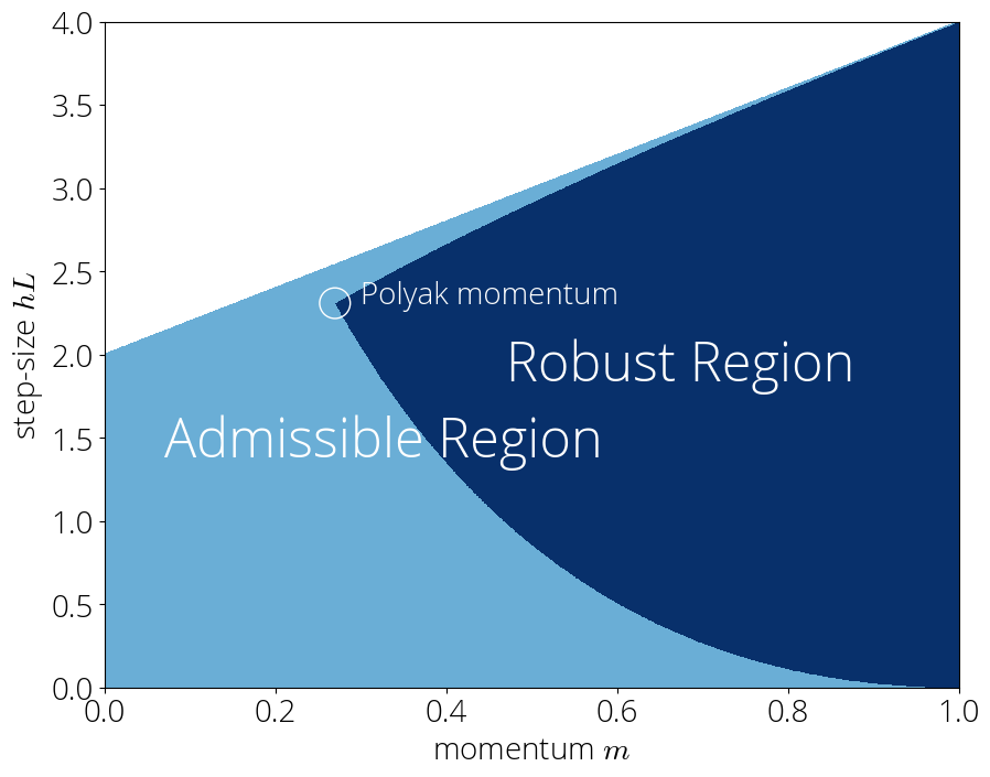\end{equation} We will refer to the set of parameters that verify the above as the robust region. This is a subset of the set of admissible parameters –that is, those for which the method converges–. The set of admissible parameters is \begin{equation} 0 \leq {\color{colormomentum}m} \lt 1 \quad \text{ and }\quad {\color{colorstepsize}h} \lt \frac{2 (1 + {\color{colormomentum}m})}{L}\,. \end{equation}

The robust region is the set of momentum (${\color{colormomentum}m}$) and step-size parameters (${\color{colorstepsize}h}$) that satisfy inequality \eqref{eq:condition_stable_region}. It's a subset of the set of parameters for which momentum converges (admissible region).

Example of robust region for $\lmin=0.1, L=1$.

In the robust region, can use the bounds above and we have the rate \begin{equation}\label{eq:convergence_rate_stable} r_t \leq {\color{colormomentum}m}^{t/2} \left( 1 + {\small\frac{1 - {\color{colormomentum}m}}{1 + {\color{colormomentum}m}}}\, t\right) \end{equation} This convergence rate is somewhat surprising, as one might expect that the convergence depends on both the step-size and momentum. Instead, in the robust region the convergence rate does not depend on the step-size. This insensitivity to step-size can be leveraged for example to develop a momentum tuner.

Given that we would like the convergence rate to be as small as possible, it's natural to choose the momentum term as small as possible while staying in the robust region. But just how small can we make this momentum term?

Polyak strikes back

This post ends as it starts: with Polyak momentum. We will see that minimizing the convergence rate while staying in the robust region will lead us naturally to this method.

Consider the inequalities that describe the robust region: \begin{equation}\label{eq:robust_region_2} \frac{(1 - \sqrt{{\color{colormomentum}m}})^2 }{{\color{colorstepsize}h}} \leq \lmin \quad \text{ and }\quad L \leq~\frac{(1 + \sqrt{{\color{colormomentum}m}})^2 }{{\color{colorstepsize}h}}\,. \end{equation} Solving for ${\color{colorstepsize}h}$ on both equations allows us to describe the admissible values of ${\color{colormomentum}m}$ as a single inequality: \begin{equation} \left(\frac{1 - \sqrt{{\color{colormomentum}m}} }{1 + \sqrt{{\color{colormomentum}m}}}\right)^2 \leq \lmin L\,. \end{equation} The left hand side is monotonicallydecreasing in ${\color{colormomentum}m}$. Since our objective is to minimize ${\color{colormomentum}m}$, this will be achieved when the inequality becomes an equality, which gives \begin{equation} {\color{colormomentum}m = {\Big(\frac{\sqrt{L}-\sqrt{\lmin}}{\sqrt{L}+\sqrt{\lmin}}\Big)^2}} \end{equation} Finally, the step-size parameter ${\color{colorstepsize}h}$ can be computed from plugging the above momentum parameter into either one of the inequalities \eqref{eq:robust_region_2}: \begin{equation} {\color{colorstepsize}h = \Big(\frac{ 2}{\sqrt{L}+\sqrt{\lmin}}\Big)^2}\,. \end{equation} These are the step-size and momentum parameter of Polyak momentum of \eqref{eq:polyak_parameters}.

This provides an alternative derivation of Polyak momentum from Chebyshev polynomials.Another way to derive Polyak momentum consists in taking the limit $t\to \infty$ of the Chebyshev iterative method derived in the previous post. See for instance paragraph "Simpler stationary recursion" in Francis' blog post. One advantage of this derivation is that we obtain the convergence rate for free. Since this combination of step-size and momentum belongs to the robust region, we can apply \eqref{eq:convergence_rate_stable}, which gives \begin{align} r_t^{\text{Polyak}} &\leq \left({\small\frac{\sqrt{L} - \sqrt{\lmin}}{\sqrt{L} + \sqrt{\lmin}}}\right)^t\left({\small 1 + t\frac{2 \sqrt{L \lmin}}{L + \lmin}}\right) \label{eq:nonasymptotic_polyak}\,. \end{align} This implies that the convergence rate of Polyak momentum –as the Chebyshev method– is asymptotically bounded as \begin{equation} \limsup_{t \to \infty} \sqrt[t]{r_t^{\text{Polyak}}} \leq {\small\frac{\sqrt{L} - \sqrt{\lmin}}{\sqrt{L} + \sqrt{\lmin}}}\,, \end{equation} which is a whopping square root factor improvement over gradient descent's $\frac{\lmax - \lmin}{\lmax + \lmin}$ convergence rate rate.

Stay Tuned

In this post we've only scratched the surface of the rich dynamics of momentum. In the next post we will explore dig deeper into the robust region and explore the other regions too.

Citing

If you find this blog post useful, please consider citing it as:

Momentum: when Chebyshev meets Chebyshev., Fabian Pedregosa, 2020

Bibtex entry:

  
    @misc{pedregosa2021residual,
      title={Momentum: when Chebyshev meets Chebyshev},
      author={Pedregosa, Fabian},
      howpublished = {\url{http://fa.bianp.net/blog/2020/momentum/}},
      year={2020}
    }
  
  

Acknowledgements. Thanks to Baptiste Goujaud for reporting many typos and making excellent clarifying suggestions, and to Nicolas Le Roux for catching some mistakes in an initial version of this post and providing thoughtful feedback.

References