Six: All of this has happened before.
Baltar: But the question remains, does all of this have to happen again?
Six: This time I bet no.
Baltar: You know, I've never known you to play the optimist. Why the change of heart?
Six: Mathematics. Law of averages. Let a complex system repeat itself long enough and eventually something surprising might occur. That, too, is in God's plan.

Battlestar Galactica *

Momentum with cyclical step-sizes has been shown to sometimes accelerate convergence, but why? We'll take a closer look at this technique, and with the help of polynomials unravel some of its mysteries.

Cyclical Heavy Ball

The most common variant of stochastic gradient descent uses a constant or decreasing step-size. However, some recent works advocate instead for cyclical step-sizes, where the step-size alternates between two or more values. In the blink of an eye, these methods have gone from esoteric to ubiquitous: they are now available in all major deep learning toolboxes,See for example TensorFlow, Flax and PyTorch implementations. and found applications beyond optimization in fields like probabilistic modeling.

The scheme that we will consider has two step-sizes $\stepzero, \stepone$, so that odd iterations use one step-size while even iterations use a different one.There are subtle differences between the various works published so far. For example, in the original work (Smith, 2017), the step-sizes take a sequence of values between $\stepzero$ and $\stepone$. The variant that we analyze takes instead two discrete step-sizes. The algorithm starts with an initial guess $\xx_0$ and produces successive approximations $\xx_1, \xx_2, \ldots$ to the minimizer of $f$ as follows:

Cyclical Heavy Ball
Input: starting guess $\xx_0$, step-sizes $0 \leq \stepzero \leq \stepone$ and momentum ${\color{colormomentum} m} \in [0, 1)$.
$\xx_1 = \xx_0 - \dfrac{\stepzero}{1 + {\color{colormomentum} m}} \nabla f(\xx_0)$
For $t=1, 2, \ldots$
\begin{align*}\label{eq:momentum_update} &\text{${\color{colorstepsize}h_t} = \stepzero$ if $t$ is even and ${\color{colorstepsize}h_t} = \stepone$ otherwise}\\ &\xx_{t+1} = \xx_t - {\color{colorstepsize}h_t} \nabla f(\xx_t)+ {\color{colormomentum} m}(\xx_{t} - \xx_{t-1}) \end{align*}

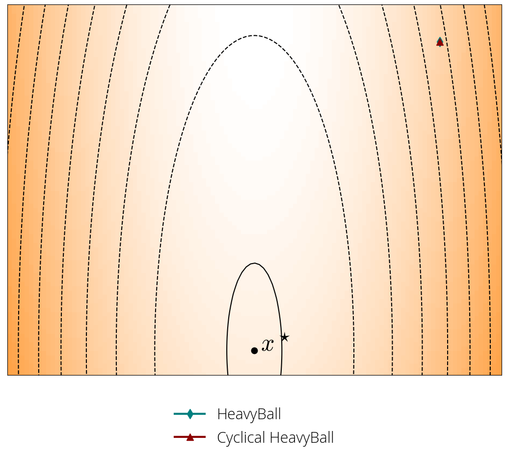
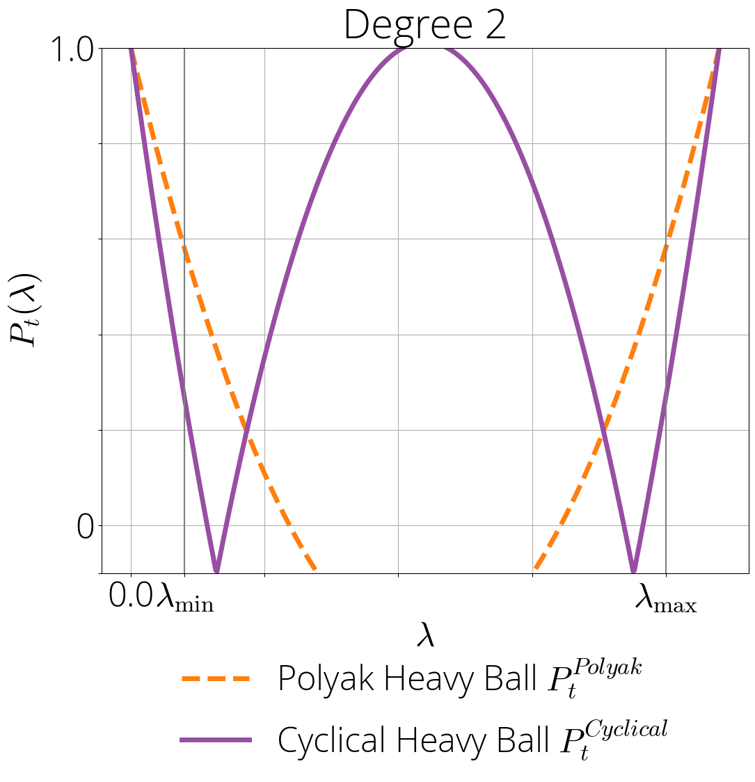
By alternating between a small and a large step-size, the cyclical step-size algorithm has very different dynamics than the classical constant step-size variant:

In both cases the parameters are set to those that maximize the asymptotic worst-case rate, assuming an imperfect lower and upper bound on the Hessian eigenvalues.

In this post, we'll show that not only the cyclical heavy-ball can reach the same convergence as optimal first-order methods such as Polyak and Nesterov momentum, but it can in fact achieve a faster convergence in some scenarios.Wait, didn't I just say that that Polyak heavy ball is optimal? How can you beat an optimal method? Hold on for a bit longer and I'll explain this apparent contradiction. We'll even be able to quantify this speedup in terms of quantities such as the eigengap, a gap in the Hessian's eigenvalues.

As in previous posts, the theory of orthogonal polynomials will be our best ally throughout the journey. We'll start by expressing the residual polynomial of the cyclical heavy ball method as a convex combination of Chebyshev polynomials of the first and second kind (Section 2), and then we'll use properties of Chebyshev polynomials to derive the worst-case optimal set of parameters (Section 3).

This post is based on a recent paper with the incredible Baptiste Goujaud, Damien Scieur, Aymeric Dieuleveut, and Adrien Taylor. The blog post only covers a subset of the results in the paper. In particular, the paper also has results on longer cycles and local convergence for non-quadratic objectives which are not covered in this blog post.

Related work

Very related to our paper is the recent work of Oymak. Here, the author derived convergence rates for gradient descent (without momentum) using a scheduler that takes one large, $K-1$ small steps instead of the alternating scheme that's the subject of this post. He showed improved convergence rates of that scheme under the same eigengap assumption we'll describe later. One important difference is that (Oymak 2021) doesn't achieve the optimal rate on general strongly convex quadratics (see Appendix E.5 ). In contrast, the method we'll describe here defaults to Polyak heavy ball and achieves the optimal rate on general quadratics.

Chebyshev Meets Cyclical Learning Rates

As in previous blog posts in this polynomials series, we'll assume our objective function $f$ is a quadratic of the form \begin{equation}\label{eq:opt} f(\xx) \defas \frac{1}{2}\xx^\top \HH \xx + \bb^\top \xx + c~, \end{equation} where $\HH$ is a $d\times d$ positive semi-definite matrix with eigenvalues in some set $\Lambda$.

As we saw in Part 2 of this series, with any gradient-based method we can associate a residual polynomial $P_t$ that will determine its convergence behavior.The notion of residual polynomial was introduced in Part 1 of this series. This association results in the following inequality that relates the error at iteration $t$ by the maximum value of the polynomial over the Hessian eigenvalue support set $\lambda$: \begin{equation} \|\xx_t - \xx^\star\| \leq {\color{purple}\underbrace{\vphantom{\max_{[L]}}\max_{\lambda \in \Lambda }}_{\text{conditioning}}} \, {\color{teal}\underbrace{\vphantom{\max_{[L]}}|P_t(\lambda)|}_{\text{algorithm}} } \,\, {\color{brown}\underbrace{\vphantom{\max_{[L]}}\|\xx_0 - \xx^\star\|}_{\text{initialization}}}~. \end{equation} This inequality highlights the importance of being able to bound the residual polynomial,We'll sometimes refer to ${\max_{\lambda \in \Lambda}|P_t(\lambda)|}$ as the convergence rate of the algorithm. as doing so results in a bound for the error norm $\|\xx_t - \xx^\star\|$, which is often the goal in the analysis of optimization algorithms. This and the next 2 sections are devoted to characterizing and bounding the residual polynomial of the cyclical heavy ball method.

Let $P_{t}$ denote the residual polynomials associated with the cyclical heavy ball method at iteration $t$. By our definition of the residual polynomial in Part 1, the sequence of residual polynomials admits the recurrence \begin{equation} \begin{aligned} &P_{t+1}(\lambda) = (1 + \mom - {\color{colorstepsize}h_{\bmod(t, 2)}} \lambda) P_{t}(\lambda) - \mom P_{t-1}(\lambda)\\ &P_0(\lambda) = 1\,,\quad P_1(\lambda) = 1 - \frac{\stepzero}{1 + \mom}\lambda\,. \end{aligned}\label{eq:residual_cyclical_recurrence} \end{equation} What makes this recurrence different than other's we'e seen before is that the terms that multiply the previous polynomials depend on the iteration number $t$ through the step-size ${\color{colorstepsize}h_{\bmod(t, 2)}}$ . This is enough to break the previous proof technique.

Luckily, we can eliminate the dependency on the iteration number by chaining iterations in a way that the recurrence jumps two iterations instead of one. Evaluating the previous equation at $P_{2t + 2}$ and solving for $P_{2t + 1}$ gives \begin{equation} P_{2t + 1}(\lambda) = \frac{P_{2t + 2}(\lambda) + \mom P_{2t}(\lambda)}{1 + \mom - \stepone\lambda}\,. \end{equation} Using this to replace $P_{2t+1}$ and $P_{2t-1}$ in the original recurrence \eqref{eq:residual_cyclical_recurrence} gives \begin{equation} \frac{P_{2t + 2}(\lambda) + \mom P_{2t}(\lambda)}{1 + \mom - \stepone\lambda} = (1 + \mom - \stepzero \lambda) P_{2t}(\lambda) - \mom \left(\frac{P_{2t}(\lambda) + \mom P_{2t-2}(\lambda)}{1 + \mom - \stepone\lambda} \right)\,, \end{equation} which solving for $P_{2t + 2}$ finally gives \begin{equation}\label{eq:recursive_formula} P_{2t + 2}(\lambda) = \left( (1 + \mom - \stepzero\lambda)(1 + \mom - \stepone \lambda) - 2 \mom \right) P_{2t}(\lambda) - \mom ^2 P_{2t - 2}(\lambda)\,. \end{equation} This recurrence expresses $P_{2t+2}$ in terms of $P_{2t}$ and $P_{2t - 2}$. It's hence a recurrence for only even iterations, but it has one huge advantage with respect to the previous one: the coefficients that multiply the previous polynomials now don't depend on the iteration number.

Once we have this recurrence, following a similar proof to the one we did in Part 2, we can derive an expression for the residual polynomial $P_{2t}$ based on Chebyshev polynomials of the first and second kind. This is useful because it will later make it easy to bound this polynomial –and develop convergence rates– using known bounds for Chebyshev polynomials.

Consider the cyclical heavy ball method with step-sizes $\stepzero$, $\stepone$, and momentum parameter $\mom$. Then the residual polynomial $P_{2t}$ of even degree associated with this method can be written in terms of Chebyshev polynomials of the first ($T_{t}$) and second kind $(U_{t})$ as \begin{align}\label{eq:theoremP2t} P_{2t}(\lambda) &= \mom^t \left( \tfrac{2 \mom}{1 + \mom}\, T_{2t}(\zeta(\lambda)) + \tfrac{1 - \mom}{1 + \mom} \, U_{2t}(\zeta(\lambda))\right)\,, \end{align} with $\zeta(\lambda) = \frac{1+\mom}{2 \sqrt{\mom}}\sqrt{(1 - \tfrac{\stepzero}{1 + \mom}\lambda)(1 - \tfrac{\stepone}{1+\mom} \lambda) }$. Since $\zeta$ is evaluated only at even polynomials, the result doesn't depend on the branch of the square root function. Note $\zeta$ can be either a real or pure imaginary number.

It's All About the Link Function

In part 2 of this series of blog posts, we derived the residual polynomial $P^{\text{HB}}_{2t}$ of (constant step-size) heavy ball. We expressed this polynomial in terms of Chebyshev polynomials as \begin{equation} P^{\text{HB}}_{2t}(\lambda) = {\color{colormomentum}m}^{t} \left( {\small\frac{2 {\color{colormomentum}m}}{1 + {\color{colormomentum}m}}}\, T_{2t}(\sigma(\lambda)) + {\small\frac{1 - {\color{colormomentum}m}}{1 + {\color{colormomentum}m}}}\, U_{2t}(\sigma(\lambda))\right)\,. \end{equation} with $\sigma(\lambda) \defas {\small\dfrac{1}{2\sqrt{{\color{colormomentum}m}}}}(1 + {\color{colormomentum}m} - {\color{colorstepsize} h}\,\lambda)$. It turns out that the above is essentially the same polynomial as the one associated with the cyclical heavy ball in the previous theorem \eqref{eq:theoremP2t}, the only difference being the term inside the Chebyshev polynomials (denoted $\sigma$ for the constant step-size and $\zeta$ for the cyclical step-size variant). We'll call these link functions.

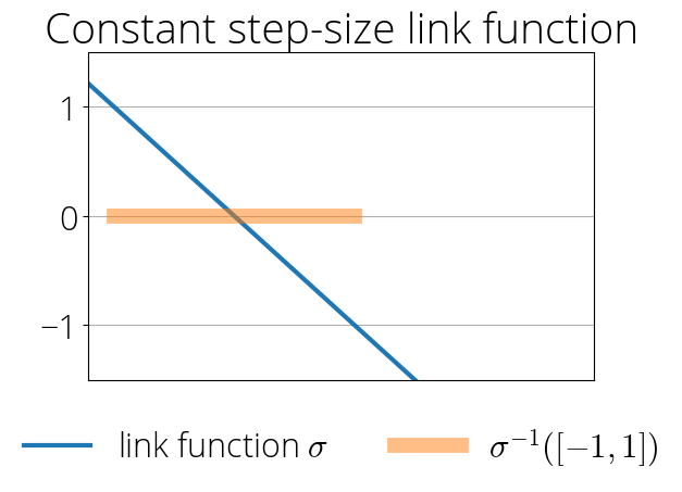
In the case of constant step-sizes, this is a linear function $\sigma(\lambda)$, while for the cyclical step-size formula is the more complicated function $\zeta(\lambda)$: \begin{align} \sigma(\lambda) &= {\small\dfrac{1}{2\sqrt{{\color{colormomentum}m}}}}(1 + {\color{colormomentum}m} - {\color{colorstepsize} h}\,\lambda) & \text{ (constant step-sizes)} \\ \zeta(\lambda) &= {\small\dfrac{1+\mom}{2 \sqrt{\mom}}}\sqrt{\big(1 - {\small\dfrac{\stepzero}{1 + \mom}}\lambda\big)\big(1 - {\small\dfrac{\stepone}{1+\mom}} \lambda\big) } & \text{(cyclical step-sizes)} \end{align} Understanding the differences between these two link functions is key to understanding cyclical step sizes.

While the link function for the constant step-size heavy ball is always real-valued, the link function of the cyclical variant is complex-valued. Hence, to provide a meaningful bound on the residual polynomial we need to understand the behaving of Chebyshev polynomials in the complex plane.

The two faces of Chebyshev polynomials

It turns out that Chebyshev polynomials always grow exponentially in the degree outside of the real segment $[-1, 1]$. In other words, Chebyshev polynomials have two clear-cut regimes: linearly bounded in $[-1, 1]$, and exponentially diverging outside.

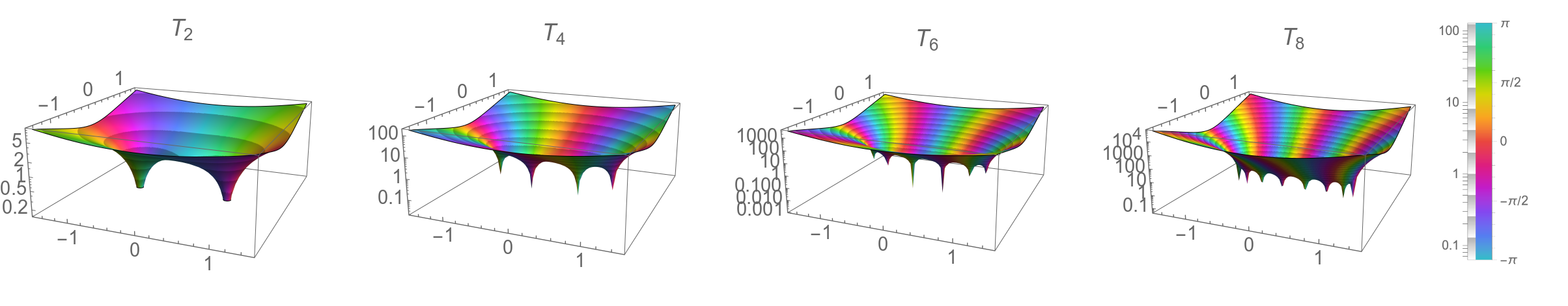
Magnitude of Chebyshev polynomials of the first kind in the complex plane. $x$ and $y$ coordinates represent the (complex) input, magnitude of the output is displayed on the $z$ axis, while the argument is represented by the color.

Zeros of Chebyshev polynomials are concentrated in the real $[-1, 1]$ segment, and the polynomials diverge exponentially fast outside it.

The following lemma formalizes this for the convex combination of Chebyshev polynomials $\frac{2{\color{colormomentum}m}}{1 + {\color{colormomentum}m}}\, T_{t}(z) + {\small\frac{1 - {\color{colormomentum}m}}{1 + {\color{colormomentum}m}}}\, U_{t}(z) $ that appear in the heavy ball method:

Let $z$ be any complex number, the sequence $ \left(\big| \small\frac{2{\color{colormomentum}m}}{1 + {\color{colormomentum}m}}\, T_{t}(z) + {\small\frac{1 - {\color{colormomentum}m}}{1 + {\color{colormomentum}m}}}\, U_{t}(z) \big|\right)_{t \geq 0} $ grows exponentially in $t$ for $z \notin [-1, 1]$, while in that interval they are bounded as $|T_t(z)| \leq 1, |U_t(z)| \leq t+1$.

A closer look into the link function

Given the previous lemma that shows that our combination of Chebyshev polynomials grows exponentially in the degree outside of $[-1, 1]$, we seek to understand when the image of the link function lies in this interval since it's in this regime where we'll expect to achieve the best rates. We'll call the set of parameters that verify this condition the robust region.We explored this region in Part 2 of this series in the context of the classical heavy ball method. The name is in reference to the step-size stability of the method: inside this region, the rate of convergence is independent of the step-sizes and only depends on the momentum term.

The link function $\sigma$ for the constant ste-size heavy ball is a linear function, so its preimage $\sigma^{-1}([- 1, 1])$ is also an interval. This explains why most analyses of the heavy ball assume the eigenvalues belonging to a single interval.

While the preimage $\sigma^{-1}([-1, 1])$ associated with the constant step-size link function is always an interval, things become more interesting for the cyclical link function $\zeta$. In this case, the preimage is not always an interval:

The preimage $\zeta^{-1}([-1, 1])$ of the cyclical step-size link function is a union of two disjoint intervals. $\zeta(\lambda)$ is larger than 1 to the left of the left interval and smaller than -1 to the right of the right interval. In between both intervals, $\zeta(\lambda)$ is purely imaginary.

For visualization purposes, we choose the branch of the square root that agrees in sign with $(1 + \mom - \stepone \lambda)$. This doesn't affect the rate, since this term only appears squared in the residual polynomial expression.

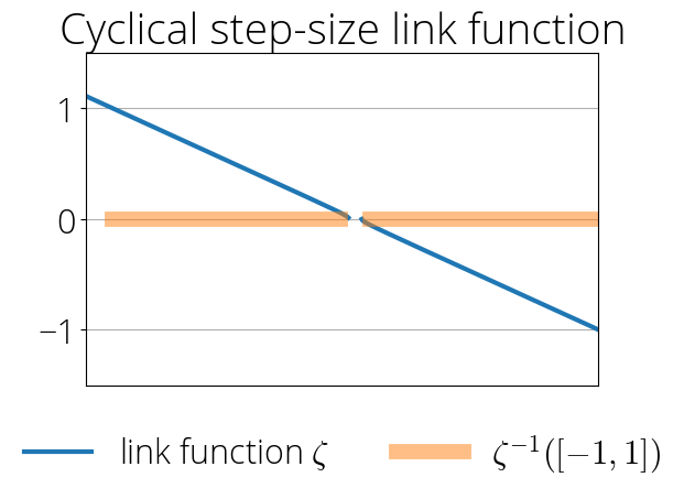
The preimage $\zeta^{-1}([-1, 1])$ associated with the cyclical step-size link function is always a union of two intervals. Chihara
Theodore Seio Chihara is known for his research in the field of orthogonal polynomials and special functions. He wrote the very influential book An Introduction to Orthogonal Polynomials. The family of Al-Salam-Chihara and Brenke-Chihara polynomials are named in his honor. worked out the exact formula for this preimage, which turns out to be a union of two intervals of the same size: \begin{equation} \begin{aligned} \zeta^{-1}([-1, 1]) = & \left[\frac{(1+\mom)(\stepzero + \stepone)-\Delta}{2 \stepzero \stepone}, \frac{1+\mom}{\stepone}\right]\\ & \bigcup \left[\frac{1+\mom}{\stepzero}, \frac{(1+\mom)(\stepzero + \stepone)+\Delta}{2 \stepzero \stepone}\right]\,, \end{aligned}\label{eq:preimage} \end{equation} with $\Delta \defas \sqrt{(1+\mom)^2 (\stepzero + \stepone)^2- 4 (1 - \mom)^2 \stepzero \stepone}$.

One of the main differences between polynomials with constant and cyclical coefficients is the behavior of their zeros. While the zeros of orthogonal polynomials with constant coefficients concentrate in an interval, those of orthogonal polynomials with varying coefficients concentrate instead on a union of two disjoint intervals. This result has profound implications. First, remember that because of the exponential divergence of Chebyshev polynomials outside the $[-1, 1]$ interval, we'd like the image of the Hessian eigenvalues to be in this $[-1, 1]$ interval. The previous result says that the eigenvalue support set that can guarantee this is no longer a single interval (as was the case for the constant step-size heavy ball) but a union of two disjoint intervals. We'll explore the implications of this model in the next section.

A Refined Model of the Eigenvalue Support Set

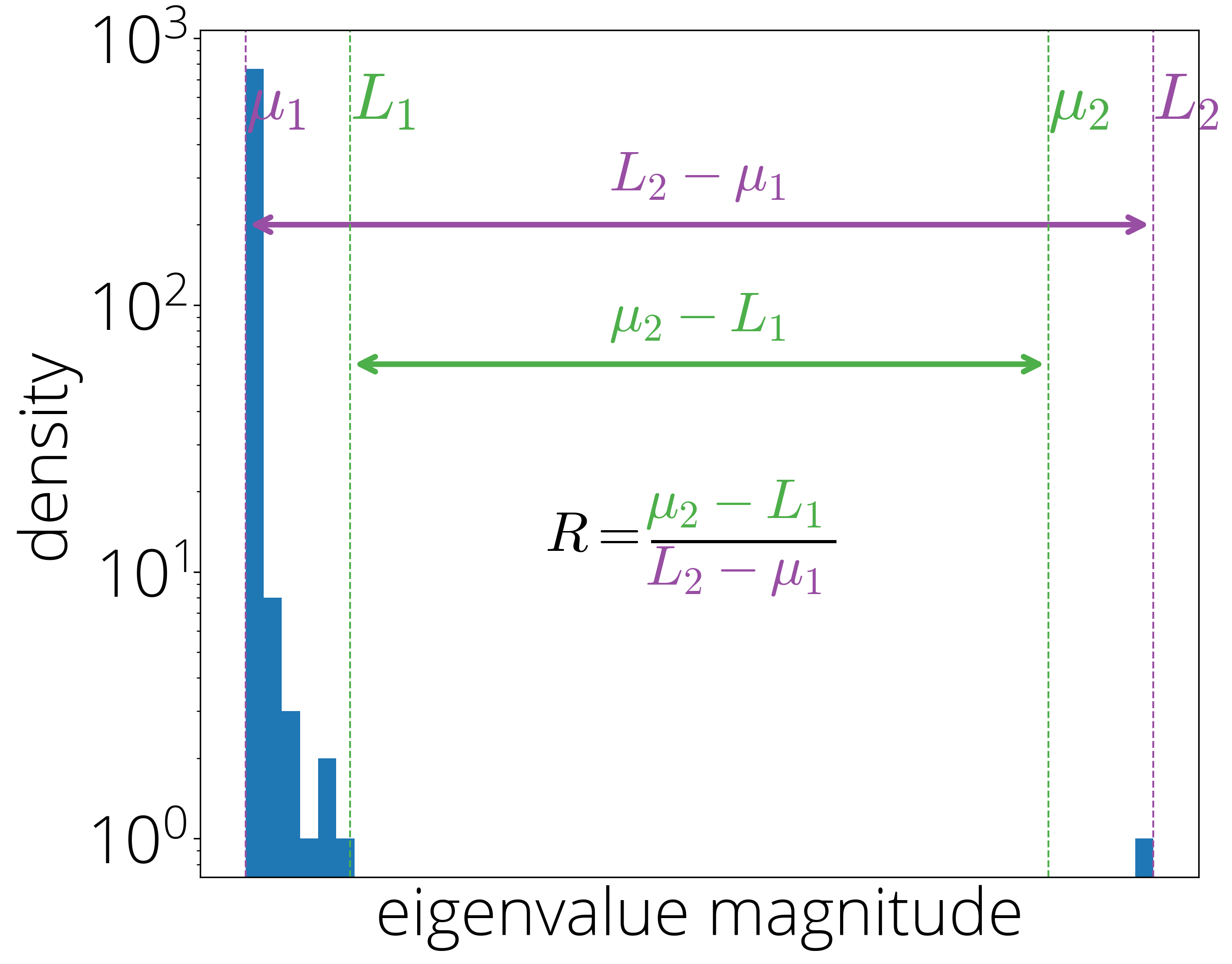
In the following we'll assume that the eigenvalues of $\HH$ lie in a set $\Lambda$ that is a union of two intervals of equal size: \begin{align} \Lambda \defas [\muone, \Lone] \cup [\mutwo, \Ltwo]\,, \end{align} with $\Lone - \muone = \Ltwo - \mutwo$. Note that this parametrization is strictly more general than the classical assumption that the eigenvalues lie within an interval since we can always take $\Lone = \mutwo$, in which case $\Lambda$ becomes the $[\muone, \Ltwo]$ interval.

A quantity that will be crucial later on is the relative gap or eigengap: \begin{equation} R \defas \frac{\mutwo - \Lone}{\Ltwo - \muone}\,. \end{equation} This quantity measures the size of the gap between the two intervals. $R=0$ implies that the two intervals are adjacent ($\Lone = \mutwo$ and the set $\Lambda$ is in practice a single interval), while $R=1$ implies instead that all eigenvalues are concentrated around the largest and smallest value.

It turns out that many deep neural networks Hessians fit into this model with a non-trivial gap. And we don't have to look too far. The venerable MNIST exhibits this behavior with a quadratic objective, which contains an outlier eigenvalue leading to a non-trivial relative gap:

Hessian eigenvalue histogram for a quadratic objective on MNIST. The outlier eigenvalue at $\Ltwo$ generates a non-zero relative gap R = 0.77. In this case, the 2-cycle heavy ball method has a faster asymptotic rate than the single-cycle one (see Section 3.2)

More complex eigenvalue structures are equally possible to model with longer cycle lengths. While we won't go into these techniques in this blog post, some are discussed in the paper.

A Growing Robust Region

The set of parameters for which the image of the link function is in the $[-1, 1]$ interval is called the robust region.We've discussed the robust region in detail in Part 3 of this series. Two of the most important properties are $i)$ the optimal convergence rate is achieved in this region, and $ii)$ the step-size doesn't influence the convergence rate in this region, which is fully determined by the momentum parameter. Using known bounds of Chebyshev polynomials $|T_t(z)| \leq 1$ and $|U_t(z)| \leq t+1$ for $z \in [-1, 1]$, we can compute the convergence rate in this region. In particular, plugging these bounds into the characterization of cyclical heavy ball's residual polynomial in Goujaud's theorem we have: \begin{equation} r_{2t} \defas \max_{\lambda \in \Lambda}|P_{2t}(\lambda)| \leq \mom^{t} \left( 1 + {\small\frac{1 - {\color{colormomentum}m}}{1 + {\color{colormomentum}m}}}\, 2 t\right)\,. \end{equation} Asymptotically, the first exponential term $\mom^{t}$ dominates, and we have the asymptotic rate \begin{equation}\label{eq:asymptotic_rate} \limsup_{t \to \infty} \sqrt[2t]{r_{2t}} = \sqrt{\mom} \end{equation}

Surprisingly, this $\sqrt{\mom}$ asymptotic rate is the same expression for constant step-size heavy ball!. It might seem we've done all this work for nothing ...

Fortunately, this is not true, our work has not been in vain. There is a speedup, but the reason is subtle. While it's true that the expression for the convergence rate is the same for constant step-size and cyclical, the robust region is not the same. Hence, the minimum momentum that we can plug in this expression is not the same, potentially resulting in a different asymptotic rate.

We now seek to find the smallest momentum parameter we can take while staying within the robust region, which is to say while the pre-image $\zeta^{-1}([-1, 1])$ contains the eigenvalue set $\Lambda$.

The area of that pre-image can be computed from the formula \eqref{eq:preimage}, and it turns out that this area factors as a product of two terms that are increasing in $\mom$: \begin{align} & \frac{\sqrt{(1+\mom)^2 (\stepone+\stepzero)^2- 4 (1 - \mom)^2 \stepzero \stepone}}{\stepzero \stepone} + (1+\mom)(\frac{1}{\stepone} - \frac{1}{\stepzero}) \\ &= \underbrace{\vphantom{\left[ \sqrt{(\stepone + \stepzero)^2 - 4 \left(\frac{1-\mom}{1+\mom}\right)^2} + \stepzero - \stepone \right]}\left[\frac{1 + \mom}{\stepzero \stepone} \right]}_{\text{positive increasing}}\underbrace{\left[ \sqrt{(\stepone + \stepzero)^2 - 4 \left(\frac{1-\mom}{1+\mom}\right)^2} + \stepzero - \stepone \right]}_{\text{positive increasing}}\,. \end{align}

The second term is increasing since $(\frac{1-\mom}{1+\mom})^2$ is decreasing, and has a minimum at $\mom=0$ where its zero. Since a product of two increasing and non-negative functions is increasing, we conclude that the area is an increasing function of $\mom$. Since the are of the robust region is increasing with $\mom$, the smallest value of $\mom$ while staying in the robust region is achieved when this region coincides with the eigenvalue support $\Lambda$.Making the region exactly coincide with the eigenvalue support set is possible thanks to the assumption that the two intervals are of the same size Hence, for the optimum momentum, the inequalities that determine the robust region become equalities, leading to the system \begin{equation} \begin{aligned} \zeta(\muone) = 1\,,\quad \zeta(\Lone) = 0 \,,\quad\\ \zeta(\mutwo) = 0 \,,\quad \zeta(\Ltwo) = -1 \,. \end{aligned} \end{equation}

From the second and third we get the optimal step-size parameters \begin{equation} \stepzero = \frac{1+\mom}{\mutwo}~,\quad \stepone = \frac{1+\mom}{\Lone}\,. \end{equation} The value of these optimal step-sizes is illustrated in the figure below, where we can see

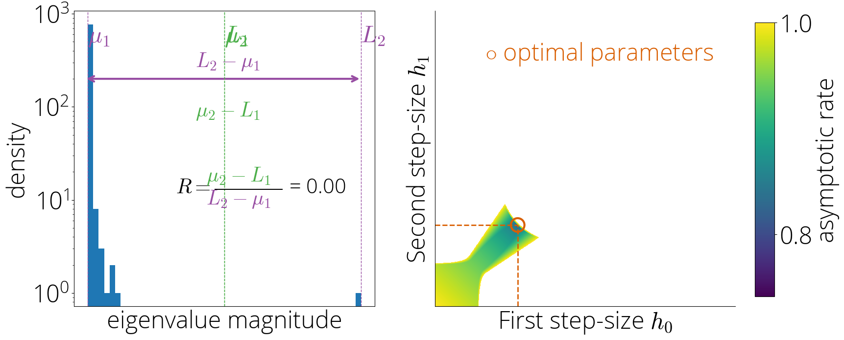
Convergence rate (in color) for every choice of step-size parameters. The optimal step-sizes are highlighted in orange.

We can see how the optimal step-sizes are identical for a trivial eigengap $(R=0)$, and grow further apart with $R$.

Replacing into the first equation (or fourth, they are redundant) and moving all momentum terms to one side we have \begin{align} \big({\small\dfrac{1 + \mom}{2 \sqrt{\mom}}}\big)^2 & = {\small\dfrac{\Lone \mutwo}{(\Lone - \muone)(\mutwo - \muone)}}\,. \end{align} Let $\rho \defas \frac{\Ltwo+\muone}{\Ltwo-\muone} = \frac{1 + \kappa}{1-\kappa}$ be the inverse of the linear convergence rate of the Gradient Descent method. With this notation, we can rewrite the above equation as \begin{equation} \Big({\small\dfrac{1 + \mom}{2 \sqrt{\mom}}}\Big)^2 = \frac{\rho^2 - R^2}{1 - R^2}\,. \end{equation} Solving for $\mom$ finally gives \begin{equation} \mom = \Big( \frac{\sqrt{\rho^2 - R^2} - \sqrt{\rho^2 - 1}}{\sqrt{1 - R^2}}\Big)^2\,. \end{equation}

With these parameters, we can now write the cyclical heavy ball method with optimal parameters. This is a method that requires knowledge of the smallest and largest Hessian eigenvalue and the relative gap $R$:

Cyclical Heavy Ball with optimal parameters
Input: starting guess $\xx_0$ and eigenvalue bounds $\muone, \Lone, \mutwo, \Ltwo$.
Set: $\rho = \frac{\Ltwo+\muone}{\Ltwo-\muone}$, $R=\frac{\mutwo - \Lone}{\Ltwo - \muone}$,
$\mom = \big( \frac{\sqrt{\rho^2 - R^2} - \sqrt{\rho^2 - 1}}{\sqrt{1 - R^2}}\big)^2$
$\xx_1 = \xx_0 - \frac{1}{\mutwo} \nabla f(\xx_0)$
For $t=1, 2, \ldots$
\begin{align*}\label{eq:momentum_update_optimal} &\text{${\color{colorstepsize}h_t} = \textstyle\frac{1+\mom}{\mutwo}$ if $t$ is even and ${\color{colorstepsize}h_t} = \textstyle\frac{1+\mom}{\Lone}$ otherwise}\\ &\xx_{t+1} = \xx_t - {\color{colorstepsize}h_t} \nabla f(\xx_t)+ {\color{colormomentum} m}(\xx_{t} - \xx_{t-1}) \end{align*}

Convergence Rates

We've seen in the previous section that in the robust region, the convergence rate is a simple function of the momentum parameter. The only thing left to do is then to plug our optimal parameter into this formula \eqref{eq:asymptotic_rate}. The following corollary provides it and an asymptotic version.

Let $x_t$ be the iterate generated by the above algorithm after an even number of steps $t$ and let $\rho \defas \frac{\Ltwo+\muone}{\Ltwo-\muone} = \frac{1 + \kappa}{1-\kappa}$ be the inverse of the linear convergence rate of the Gradient Descent method. Then we can bound the iterate suboptimality by a product of two terms, the first of which decreases exponentially fast, while the second one increases linearly in $t$: \begin{equation} \frac{\|x_t - x_\star\|}{\|x_0 - x_\star\|} \leq \underbrace{\vphantom{\sum_i}\textstyle\Big(\frac{\sqrt{\rho^2 - R^2} - \sqrt{\rho^2 - 1}}{\sqrt{1 - R^2}}\Big)^{t} }_{\text{exponential decrease}} \, \underbrace{\Big( 1 + t\sqrt{\small\dfrac{\rho^2-1}{\rho^2 - R^2}}\Big)}_{\text{linear increase}}\,. \end{equation} Asymptotically, the exponential term dominates, and we have the following asymptotic rate factor: \begin{equation} \label{eq:cyclic_rate} \limsup_{t \to \infty} \sqrt[2t]{\frac{\|x_{2t} - x_\star\|}{\|x_0 - x_\star\|}} \leq \frac{\sqrt{\rho^2 - R^2} - \sqrt{\rho^2 - 1}}{\sqrt{1 - R^2}}\,. \end{equation}

How do these compare with those of the constant step-size heavy ball method with optimal parameters (Polyak heavy ball)? The asymptotic rate of Polyak heavy ball is $r^{\text{PHB}} \defas \rho - \sqrt{\rho^2 - 1}$, and so we'd like to compare \begin{equation}\label{eq:polyak_rate} \begin{aligned} &r^{\text{CHB}} = \frac{\sqrt{\rho^2 - R^2} - \sqrt{\rho^2 - 1}}{\sqrt{1 - R^2}} \\ \text{vs } &r^{\text{PHB}} \defas \rho - \sqrt{\rho^2 - 1}\,. \end{aligned} \end{equation}

The first thing we can say is that both coincide when $R=0$, and that $r^{\text{CHB}}$ is a decreasing function of $R$, so the rate improves with the relative gap. Other than that, it's not clear how to summarize the improvement by a simpler formula.

On the ill-conditioned regime, where the inverse condition number goes to zero ($\kappa \defas \tfrac{\mu}{L} \to 0$), which is also the main case of interest, we'll be able to provide an approximation that sheds some light. In this regime, we have the following rates (lower is better): The asymptotic rate of gradient descent in this regime is $1 - 2 \kappa + o(\kappa)$. \begin{align} &r^{\text{PHB}} \underset{\kappa \rightarrow 0}{=} 1 - 2\sqrt{\kappa} + o(\sqrt{\kappa}) \\ &r^{\text{CHB}} \underset{\kappa \rightarrow 0}{=} 1 - 2\frac{\sqrt{\kappa}}{{\color{red}\sqrt{1-R^2}}} + o(\sqrt{\kappa})\,,\label{eq:approx} \end{align} where $o(\sqrt{\kappa})$ contains which to go zero faster than $\sqrt{\kappa}$ as $\kappa \rightarrow 0$. This sheds some light on the improvement: the cyclical scheduler allows us to divide the complexity of the method by a factor of $\frac{1}{\color{red}\sqrt{1-R^2}}\,$!

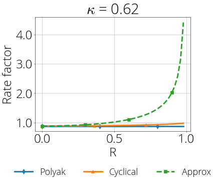
The figure below compares the convergence rate of Polyak heavy ball (Polyak), the cyclical heavy ball (Cyclical) and its approximated rate \eqref{eq:approx} (Approx, in dashed lines). We see Cyclical behaving like Polyak for well-conditioned problems (small $\kappa$) and then fitting more the super-accelerated rate (Approx) for ill-conditioned problems. This plot also shows that the approximated rate is a very good approximation for $\kappa \lt 0.001$.

Convergence rate comparison between Polyak heavy ball, Cyclical heavy ball, and its approximate convergence rate.

We can see how the approximated rate provides an excellent fit in the ill-conditioned regime.

Conclusion and Perspectives

In this post, we've shown that cyclical learning rates provide an effective and practical way to leverage a gap or bi-modal structure in the Hessian's eigenvalues. We've also derived optimal parameters and shown that in the ill-conditioned regime, this method achieves an extra rate factor improvement of $\frac{1}{\color{red}\sqrt{1-R^2}}$ over the accelerated rate of Polyak heavy ball, where $R$ is the relative gap in the Hessian eigenvalues.

The combination of a structured Hessian, momentum and cyclical learning rates is immensely powerful, and here we're only scratching the surface of what's possible. Many important cases have not yet been studied, such as the non-quadratic setting (strongly convex, convex, and non-convex). In the paper we have empirical results logistic regression showing speedup of the cyclical heavy ball method, but no proof beyond local convergence. Equally open is the extension to stochastic algorithms.

Citing

If you find this blog post useful, please consider citing as

Cyclical Step-sizes, Baptiste Goujaud and Fabian Pedregosa, 2022

with bibtex entry:

  
    @misc{goujaud2022cyclical,
      title={Cyclical Step-sizes},
      author={Goujaud, Baptiste and Pedregosa, Fabian},
      howpublished = {\url{http://fa.bianp.net/blog/2022/cyclical/}},
      year={2022}
    }
  
  

To cite its accompanying full-length paper, please use:

Super-Acceleration with Cyclical Step-sizes, Baptiste Goujaud, Damien Scieur, Aymeric Dieuleveut, Adrien Taylor, Fabian Pedregosa. Proceedings of The 25th International Conference on Artificial Intelligence and Statistics, 2022

Bibtex entry:

  
    @inproceedings{goujaud2022super,
      title={Super-Acceleration with Cyclical Step-sizes},
      author={Goujaud, Baptiste and Scieur, Damien and Dieuleveut, Aymeric and Taylor,
        Adrien and Pedregosa, Fabian},
      booktitle = {Proceedings of The 25th International Conference on Artificial
        Intelligence and Statistics},
      series = {Proceedings of Machine Learning Research},
      year={2022}
    }
  
  

References